Emily Groom, Regan Hart, Kaden Strom, Taylor Rehovsky
Stat 330
PROPOSAL
Data Set 4
In this project we would like to study the quantity of red and yellow skittles in each bag. First, we will
collect 10 bags of skittles. Then, we will count and record the quantity of the red and yellow skittles in
each bag. Next, we will study to see if one color of skittle is more dominant than the other color. The
resources that have been chosen are 10 bags of Wrigley’s Mars Skittles purchased at a convenience store
in Fargo, North Dakota.
PHASE ONE
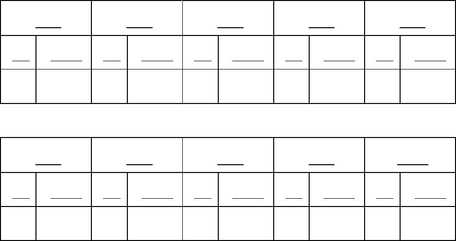
Data was collected from 10 different bags of Wrigley’s Mars Skittles that were purchased at a
convenience store in Fargo, North Dakota. The data from each bag is listed below.
Bag 1
Bag 2
Bag 3
Bag 4
Bag 5
Red
Yellow
Red
Yellow
Red
Yellow
Red
Yellow
Red
Yellow
8
6
10
11
7
12
8
9
9
10
Bag 6
Bag 7
Bag 8
Bag 9
Bag 10
Red
Yellow
Red
Yellow
Red
Yellow
Red
Yellow
Red
Yellow
7
13
5
7
10
11
11
9
9
11
When we constructed the frequency table for the Red Skittles data we first sorted the data numerically to
be able to locate the range and find the components of the frequency table easily.
1. To find the range we subtracted the smallest number of red skittles from the largest number of red
skittles.
a. 11-5 = 6, range is equal to 6.
2. We used 4 classes to represent the data, so to find the class width we took the range divided by
the number of classes.
a. 6/4 = 1.5, which we will round up to 2, giving us a class width is equal to 2.
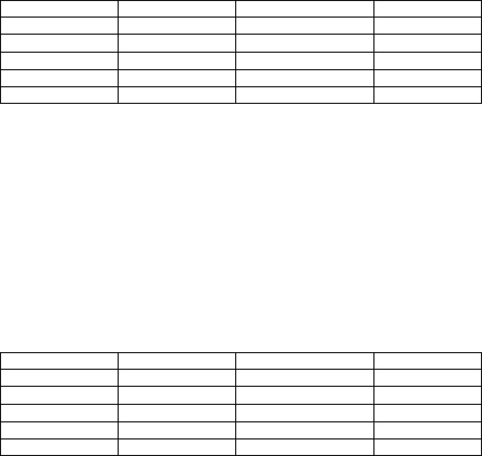
3. To find our classes we will take the smallest value and add 2 to get the second lower class limit.
We will keep adding our class width value of 2 until we achieve 4 lower class limits. From there
we will subtract one from the second lower class limit to get the upper class limit. After that we
will add 2 again until we achieve the 4th upper class limit. We will then take account for
however many observations are in each class and follow up with calculating the cumulative and
relative frequencies.
Classes
Frequency
Cumulative Frequency
Relative Frequency
5-6
1
1
0.1
7-8
4
5
0.4
9-10
4
9
0.4
11-12
1
10
0.1
10
1.00
Similar to how we found the contents for the frequency table for the Red Skittles, we will now find the
information for the Yellow skittles.
1. To find the range we subtracted the smallest number of yellow skittles from the largest number of
yellow skittles.
a. 13-6 = 7, range is equal to 7.
2. Next we found the class widths by dividing the range by the number of classes. We decided on
blank classes to represent the data.
a. 7/4 = 1.75, which we will round up to 2, giving us a class width of 2.
3. Lastly to find the upper and lower limits of our classes we took our smallest entry and added our
width to that, we did that for all of the classes to find the lower limit. To find the upper limit we
took our second smallest class and subtracted 1 from it, and that became the upper limit to the
first class. We continued that for all of the remaining classes. We then took account for however
many observations are in each class and follow up with calculating the cumulative and relative
frequencies.
Classes
Frequency
Cumulative Frequency
Relative Frequency
6-7
2
2
0.2
8-9
2
4
0.2
10-11
4
8
0.4
12-13
2
10
0.2
10
1.00
After constructing the Frequency Tables for the two sets of data, we will now construct Histograms for
the data sets.
To construct the histogram for the Red Skittles data we will take the first lower class limit and add 0.5 for
each class. This will create a midpoint for the class. These class boundaries are the horizontal, or x, scale
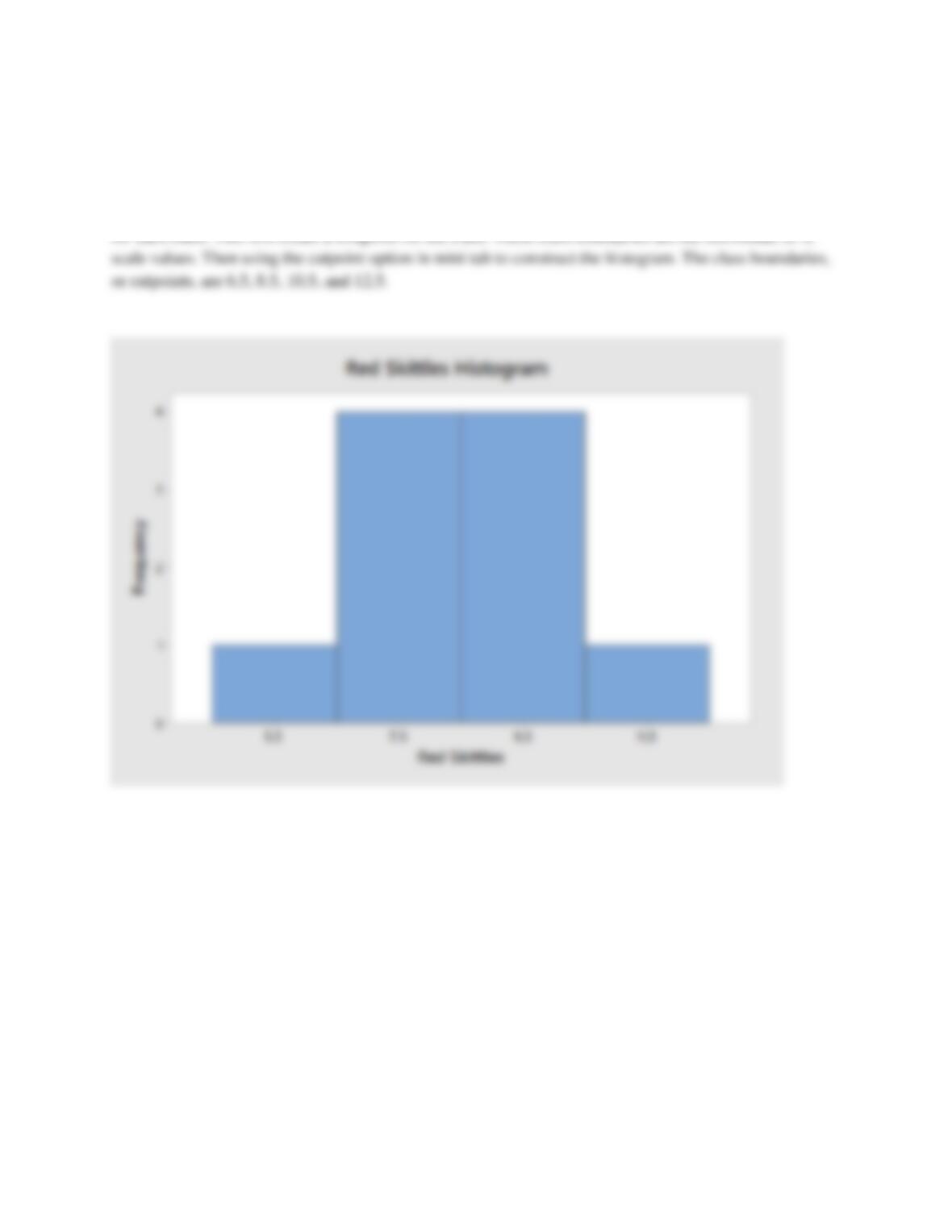
values. Then using the cutpoint option in mini tab to construct the histogram. The class boundaries, or
cutpoints, are 5.5, 7.5, 9.5, and 11.5.
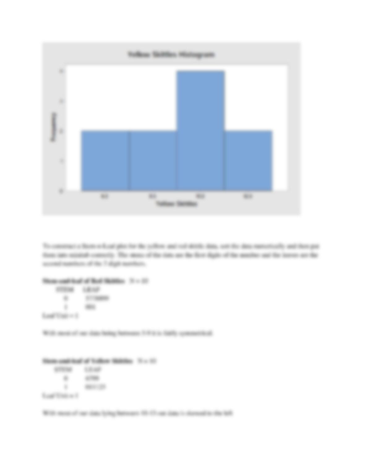
To construct the histogram for the Yellow Skittles data we will take the first lower class limit and add 0.5