Chapter 11 Aggregate Planning
2010/06/30 1
2010/06/30 2
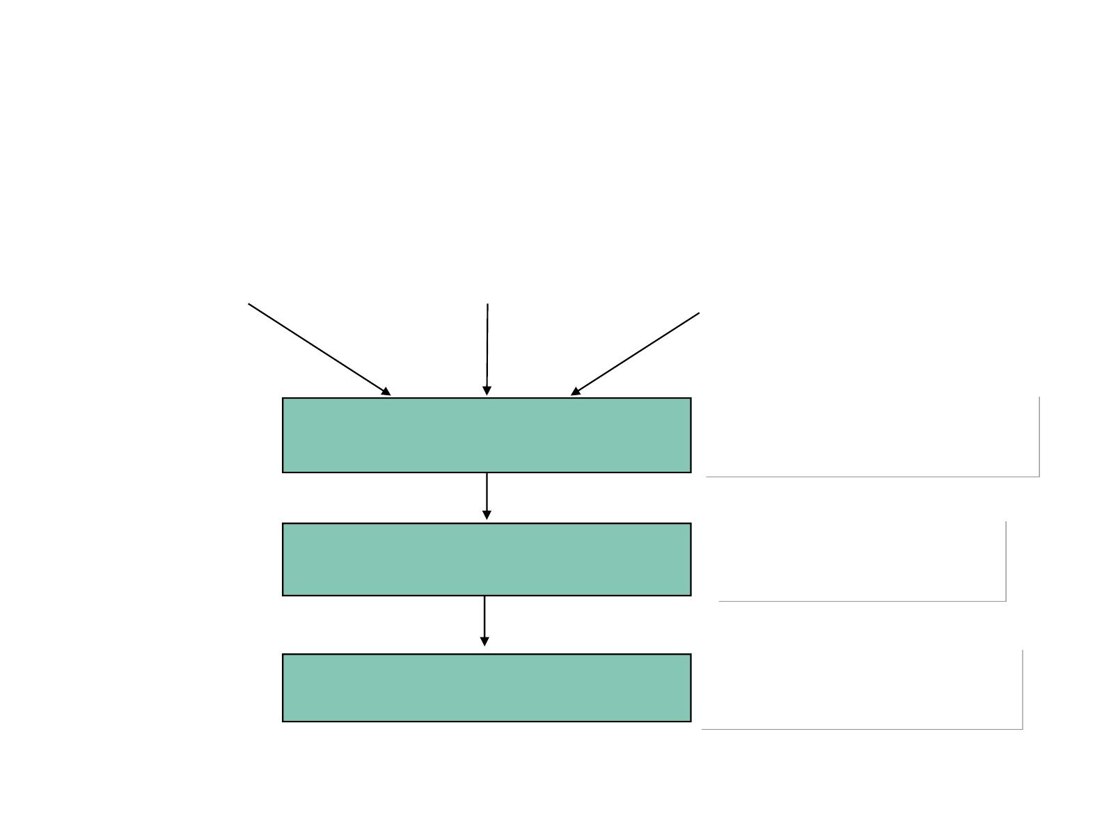
Planning Sequence
Corporate
strategies
Industry &
Environmental
Conditions
Aggregate
demand
forecasts
Business/Strategic Plan
Aggregate Production plan
Master schedule
Establishes production
and capacity strategies
Establishes
production capacity
Establishes schedules
for specific products

2010/06/30 3
•Long-range plans (typically 5 years or more)
–Long term capacity
–Location / layout
•Intermediate plans (General or aggregate levels, 2-12 months)
–Employment
–Output
•Short-range plans (Detailed plans, <=1 month)
–Machine loading
–Job assignments
Overview of Planning Levels

2010/06/30 4
What is Aggregate Planning?
•Intermediate-range capacity planning in aggregate measures, usually
covering 2 to 12 months.
•Aggregate Measures:
–No distinction between different skills
–No distinction between different models
–Examples: dollars, full-time equivalent person-years, generic units
•Central issue: What is the best (i.e., the lowest cost) way to
satisfy the demand, subject to capacity constraints?
2010/06/30 5
0
1
2
3
4
5
6
7
8
9
10
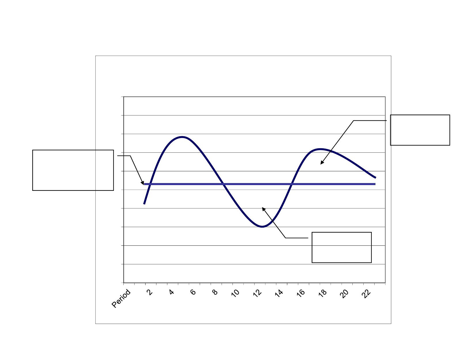
Demand
Aggregate Planning Strategies: Level
Building
inventory
Depleting
inventory
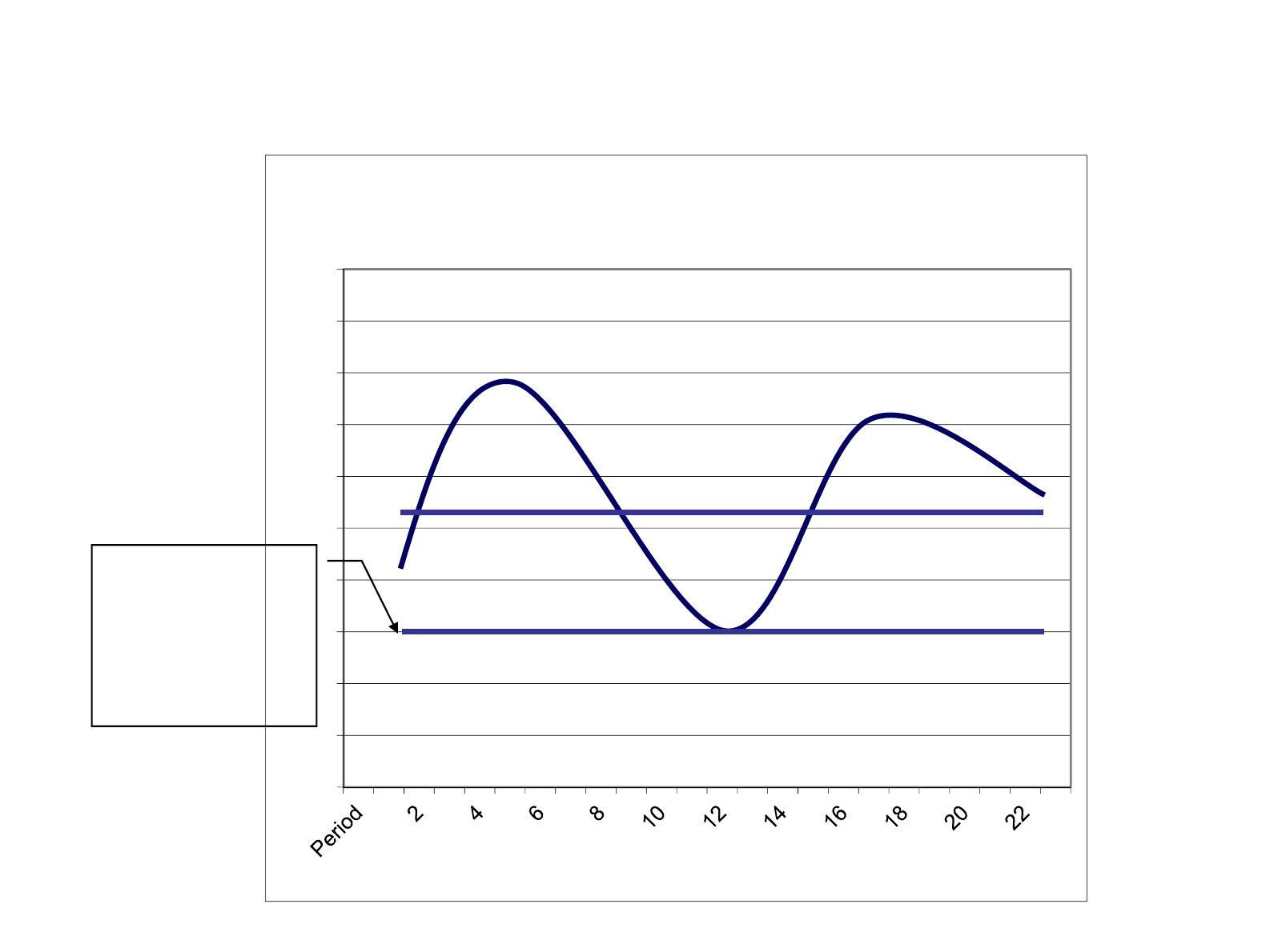
Capacity = avg
•Low idle time
•High inventory
2010/06/30 6
0
1
2
3
4
5
6
7
8
9
10
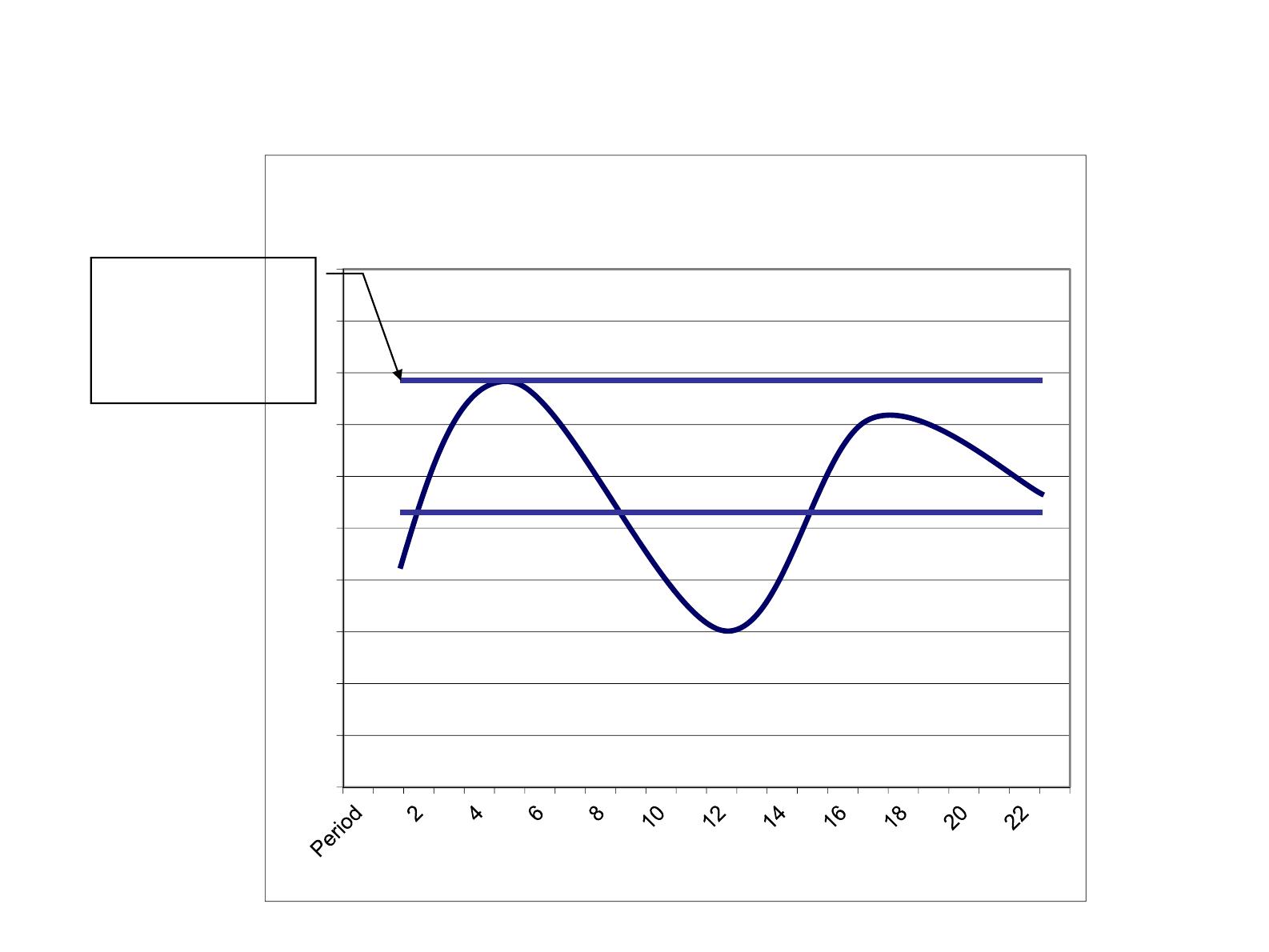
Demand
Aggregate Planning Strategies : Level
Capacity = max
•Fast response
•Excess idle
time
2010/06/30 7
0
1
2
3
4
5
6
7
8
9
10
Demand
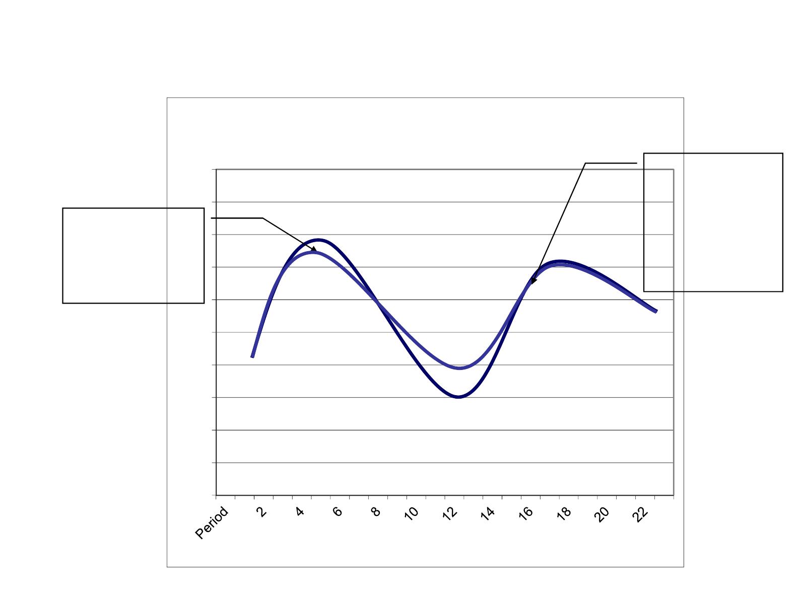
Aggregate Planning Strategies : Level
Capacity = min
•Low idle time
& greater
flexibility
•High overtime
2010/06/30 8
0
1
2
3
4
5
6
7
8
9
10
Demand
Aggregate Planning Strategies : Chase
Match capacity
with demand
within
constraints
•Low inventory/
backorder
•High capacity
variation costs
(overtime,
hire/layoff)

2010/06/30 9
Aggregate Planning Strategies
•Level Strategy
–Maintain a level workforce
–Maintain a steady output rate
•Chase Strategy:
–Match demand period by period
•Mixed Strategy:
–Use a combination of decision
variables

2010/06/30 10
•Demand forecast
•Resources
–Workforce
•Regular
•Overtime
–Subcontracting
–Facilities & equipment (given)
•Policies
–Capacity limits
–Inventory requirements
–Back orders
•Costs
–Production costs
•Regular
•Overtime
•Subcontracting
–Inventory carrying
–Back orders
–Hiring/firing
Aggregate Planning Inputs and Decision Variables

2010/06/30 11
•Planned levels of capacity
–Output from each source
–Employment
–Subcontracting
•Projected levels of inventory
–Beginning/ending, and average inventory levels
–Backorder (negative inventory)
•Costs
–Regular and overtime
–Hire and layoff
–Subcontracting
–Inventory holding and backorder
Aggregate Planning Outputs
2010/06/30 12
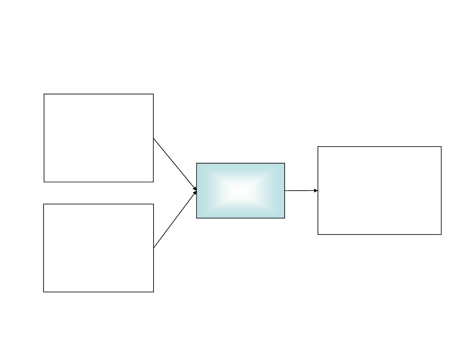
Aggregate Planning Process
Aggregate
Planning
Decisions:
•Reg. & overtime
•Subcontracting
•Hires/layoffs Plans:
•Capacity & hire/layoff
•Subcontracting
•Inventory projections
•Costs
Inputs:
•Demand forecast
•Capacity limits
•Inventory
constraints
•Unit costs
2010/06/30 13
Example: Solved Problem
PERIOD 1 2 3 4 5 6 7 8 9 TOTAL
FORE 190 230 260 280 210 170 160 260 180 1940
OUTPUT
Regular 210 210 210 210 210 210 210 210 210 1890
Overtime 0
Subcontract. 20 20 10 50
Output-Fore. 40 0 -40 -70 0 40 50 -50 30
INVENTORY
Beg. Inventory 0 40 40 0 0 0 0 20 0
End. Inventory 40 40 0 0 0 0 20 0 0
Avg. Inventory 20 40 20 0 0 0 10 10 0 100
Backorder 0 0 0 70 70 30 0 30 0 200
UNIT COSTS: TOTAL COSTS:
Regular = $6.00 /unit Regular = 11,340 TOTAL = 14,240
Overtime = $9.00 /unit Overtime = 0
Subcon. = $8.00 /unit Subcon. = 400
Holding = $5.00 /unit/period Holding = 500
Backorder = $10.00 /unit/period Backorder = 2,000
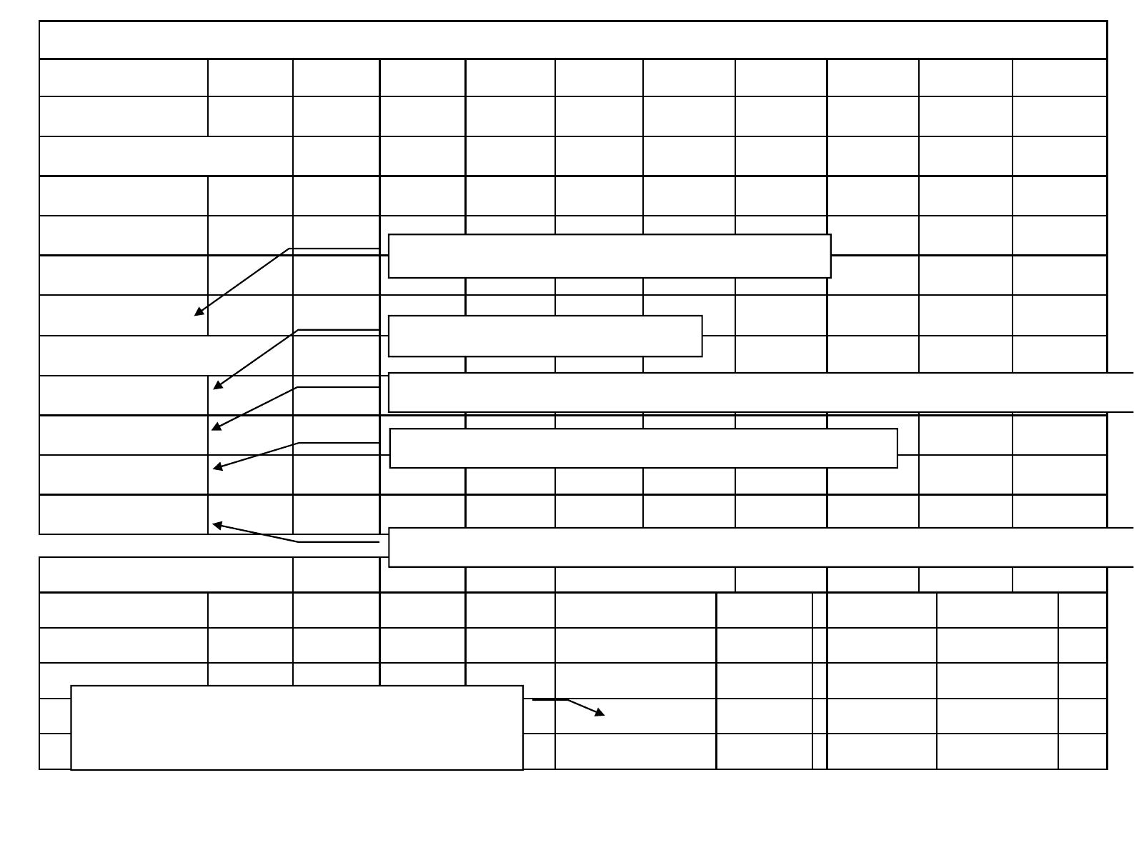
Output-Fore=Reg+OT+Sub-Fore
BegInv(t)=EngInv(t-1)
EndInv(t)=BegInv(t)+(Output-Fore)-BO(t-1) if positive, or 0
AvgInv(t)=[BegInv(t)+EndInv(t)] ÷2
BO(t)=-BegInv(t)-(Output-Fore)+BO(t-1) if positive, or 0
Total Holding Cost =
Total AvgInv * Holding/unit/period
2010/06/30 14
Example: Solved Problem
PERIOD 1 2 3 4 5 6 7 8 9 TOTAL
FORE 190 230 260 280 210 170 160 260 180 1940
OUTPUT
Regular 210 210 210 210 210 210 210 210 210 1890
Overtime 0
Subcontract. 20 20 10 50
Output-Fore. 40 0 -40 -70 0 40 50 -50 30
INVENTORY
Beg. Inventory 0 40 40 0 0 0 0 20 0
End. Inventory 40 40 0 0 0 0 20 0 0
Avg. Inventory 20 40 20 0 0 0 10 10 0 100
Backorder 0 0 0 70 70 30 0 30 0 200
UNIT COSTS: TOTAL COSTS:
Regular = $6.00 /unit Regular = 11,340 TOTAL = 14,240
Overtime = $9.00 /unit Overtime = 0
Subcon. = $8.00 /unit Subcon. = 400
Holding = $5.00 /unit/period Holding = 500
Backorder = $10.00 /unit/period Backorder = 2,000
2010/06/30 15
Example: Solved Problem
PERIOD 1 2 3 4 5 6 7 8 9 TOTAL
FORE 190 230 260 280 210 170 160 260 180 1940
OUTPUT
Regular 215 215 215 215 215 215 215 215 215 1935
Overtime 0
Subcontract.
Output-Fore. 25 -15 45 -65 5 45 55 -45 35
INVENTORY
Beg. Inventory 0 25 10 35 0 0 20 75 30
End. Inventory 25 10 35 0 0 20 75 30 65
Avg. Inventory 12.5 17.5 22.5 0 0 10 47.5 52.5 47.5 210
Backorder 0 0 0 30 25 000055
UNIT COSTS: TOTAL COSTS:
Regular = $6.00 /unit Regular = 11,610 TOTAL = 14,240
Overtime = $9.00 /unit Overtime = 0Dusan 13,900
Subcon. = $8.00 /unit Subcon. = 0
Holding = $5.00 /unit/period Holding = 1,050 13,210
Backorder = $10.00 /unit/period Backorder = 550

2010/06/30 16
•Example 1
•Example 2
•Exercise 8 and 9
Aggregate Planning

2010/06/30 17
•Table 11.5 General model
•Table 11.6 Example
Transportation Notation for
Aggregate Planning

2010/06/30 18
•Influencing the quantity of demand:
–Pricing
–Promotion
•Influencing the timing of demand
–Inventory (produce before demand occurs)
–Backorders (produce after demand occurs)
•New demand
–New market
–New market segment
Demand Management Options

2010/06/30 19
•Hire and layoff workers
•Overtime/slack time
•Part-time workers
•Changing the timing of capacity requirements
–Inventory (produce before demand occurs)
–Backorders (produce after demand occurs)
•Subcontracting
Capacity Options

2010/06/30 20
•Determine demand for each period
•Identify policies and constraints that are pertinent
•Determine capacities available for each period
•Determine units costs
•Develop alternative plans and costs
•Select the best plan that satisfies objectives
Techniques for Aggregate Planning

2010/06/30 21
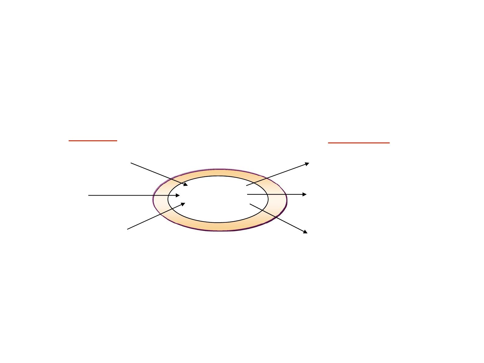
•Master schedule: The result of disaggregating an aggregate plan;
shows quantity and timing of specific end items for a scheduled
horizon.
–Figure 11.5: Disaggregating the aggregate plan
•Rough-cut capacity planning: Approximate balancing of
capacity and demand to test the feasibility of a master schedule.
Disaggregating
2010/06/30 22
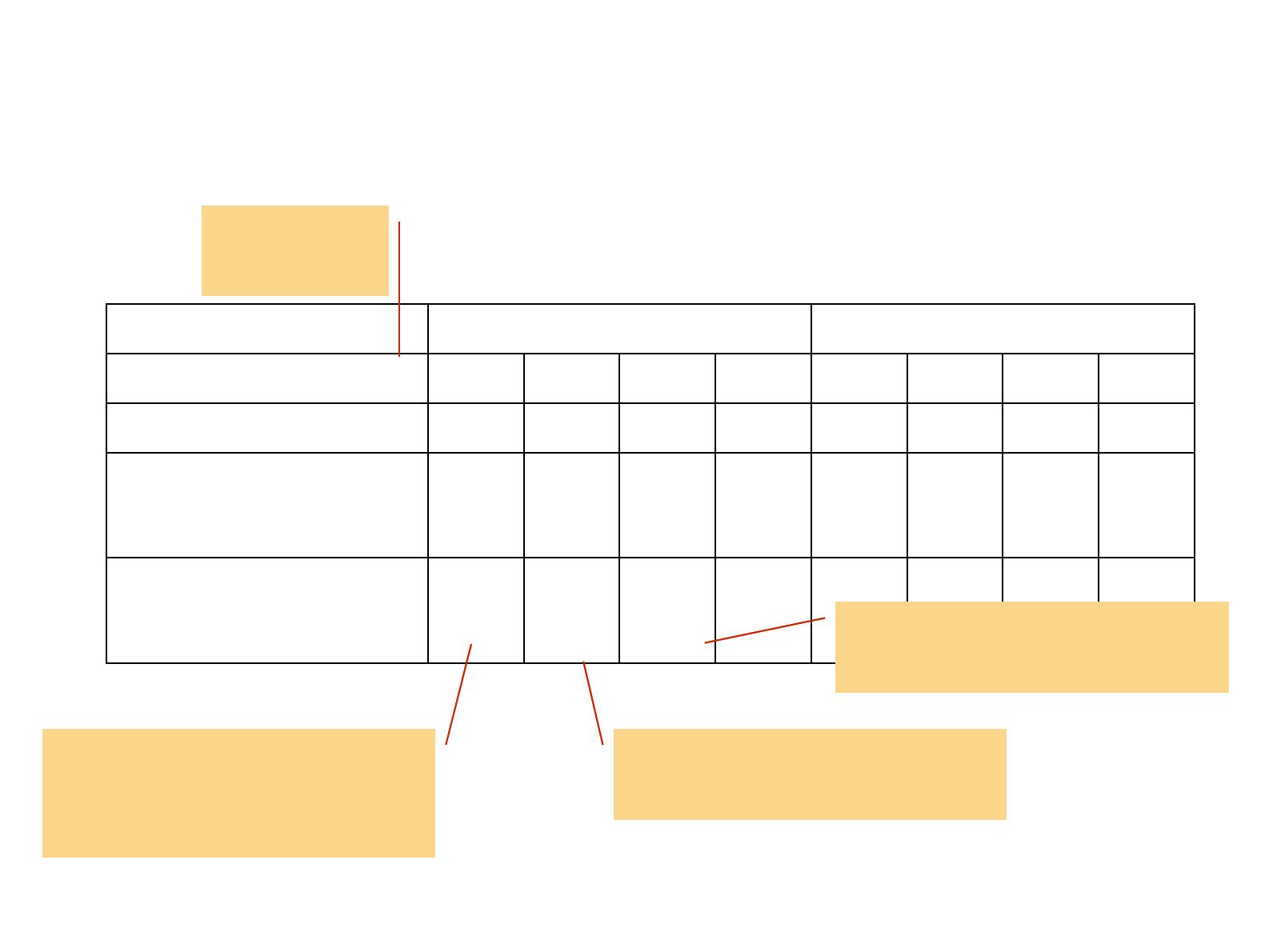
Master Scheduling Process
Master
Scheduling
Beginning inventory
Forecast
Customer orders
Inputs Outputs
Projected inventory
Master production schedule
Uncommitted inventory
2010/06/30 23
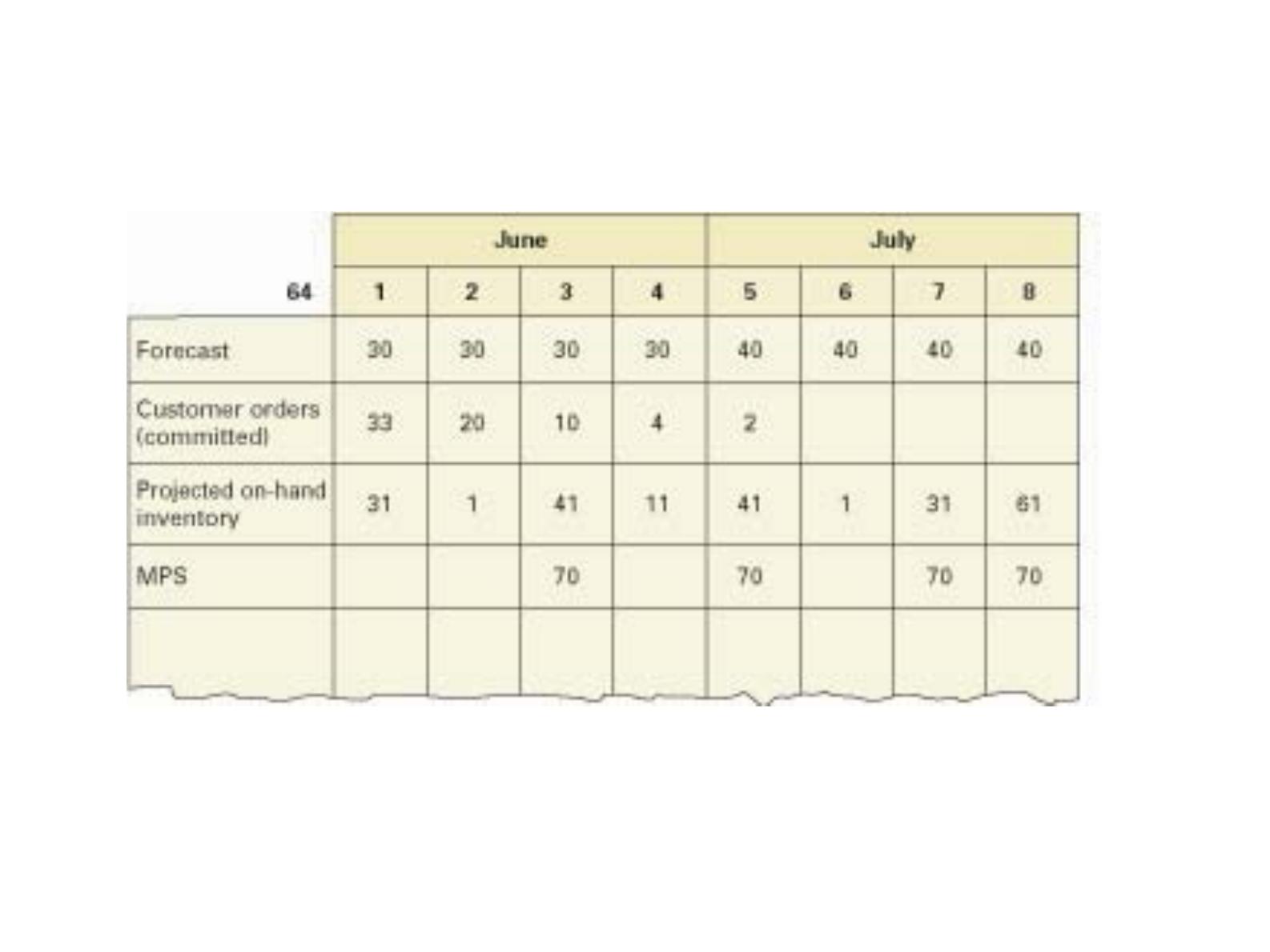
Projected On-hand Inventory
6412345678
Forecast 30 30 30 30 40 40 40 40
Customer Orders
(committed) 33 20 10 4 2
Projected on-hand
inventory 31 1 -29
JUNE JULY
Beginning
Inventory
Customer orders are
larger than forecast in
week 1
Forecast is larger than
Customer orders in week 2
Forecast is larger than
Customer orders in week 3
2010/06/30 24
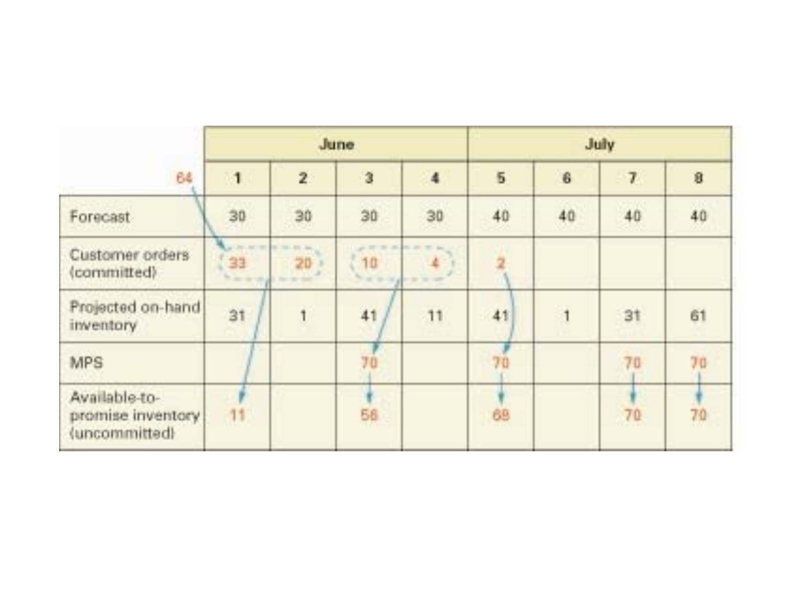
Adding MPS and Projected On Hand to the MPS
2010/06/30 25
Available to Promise

2010/06/30 26
•Exercise 21
Exercises
2010/06/30 27
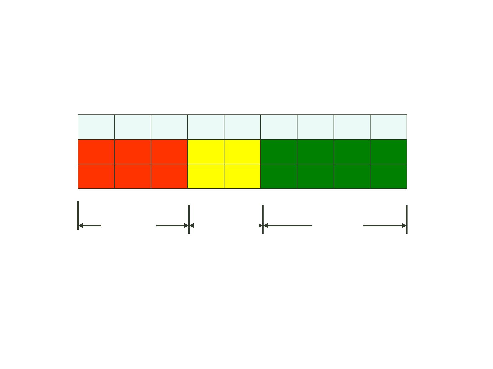
Time Fences
Period
“frozen”
(firm or
fixed)
“slushy”
somewhat
firm
“liquid”
(open)
123456789
2010/06/30 28
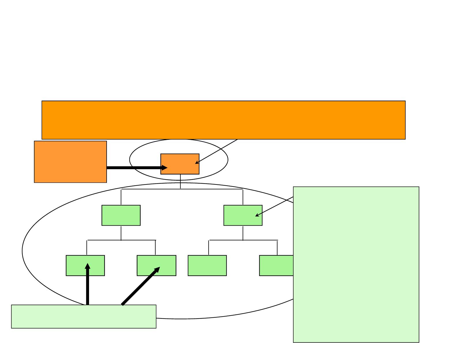
E(1
)
Independent Demand (Demand for the final end-
product or demand not related to other items)
Dependent
Demand
(Derived demand
items for
component
parts,
subassemblies,
raw materials,
etc)
Finished
product
Component parts
Material requirements planning (MRP)
•Computer-based information system for ordering and scheduling of
dependent demand inventories
•Demand for items that are subassemblies or component parts to be used in
production of finished goods.
2010/06/30 29
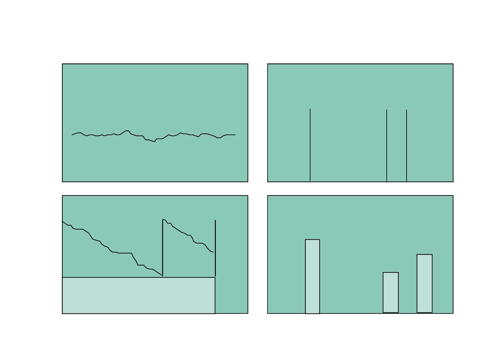
Dependent vs Independent Demand
Time
Time Time
Time
Demand
Demand
Stable demand “Lumpy” demand
Amount on hand
Amount on hand
Safety stock
2010/06/30 30
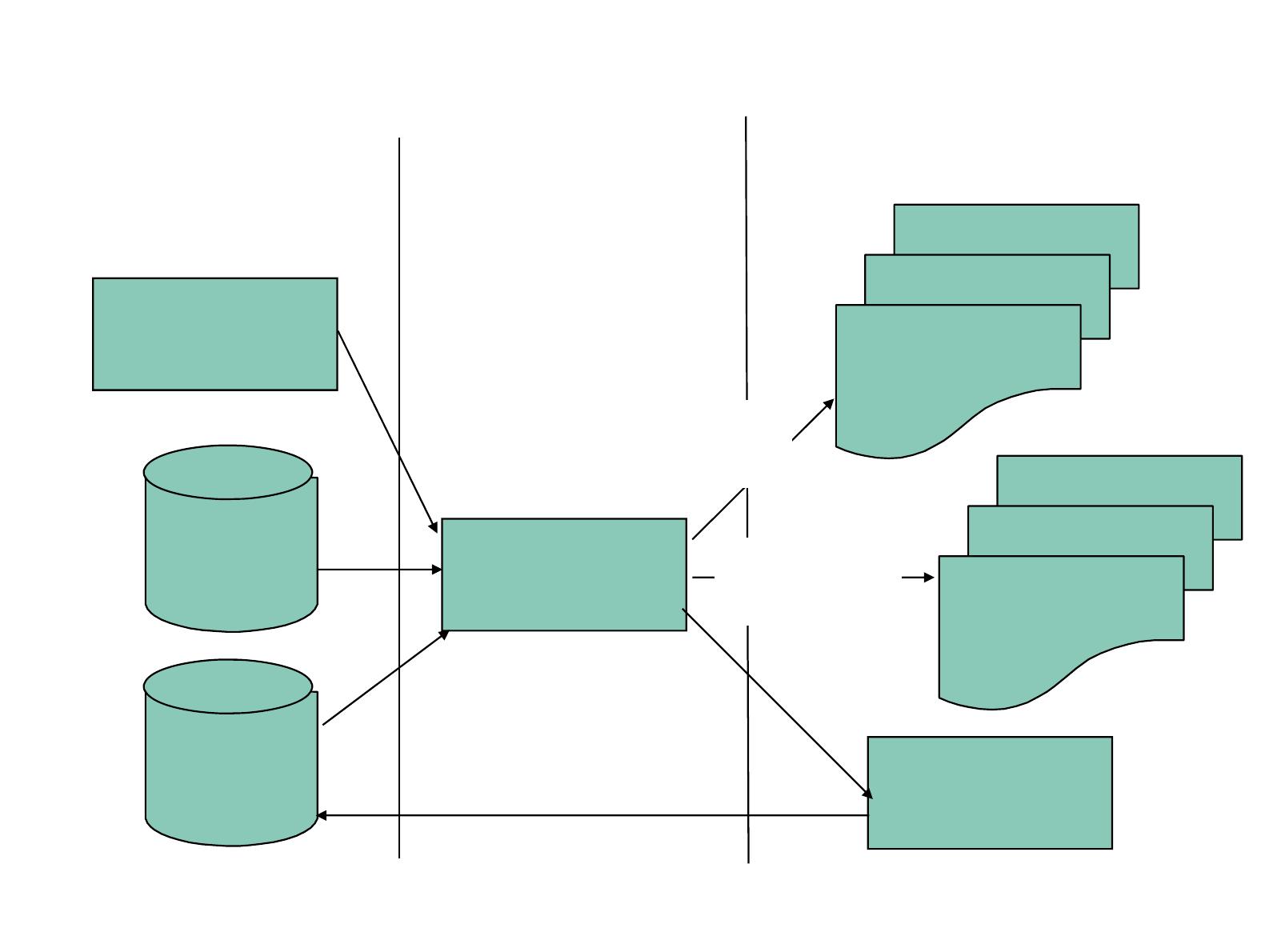
MRP Inputs MRP Processing MRP Outputs
Master
schedule
Bill of
materials
Inventory
records
MRP computer
programs
Changes
Order releases
Planned-order
schedules
Exception reports
Planning reports
Performance-
control
reports
Inventory
transaction
Primary
reports
Secondary
reports
Overview of MRP
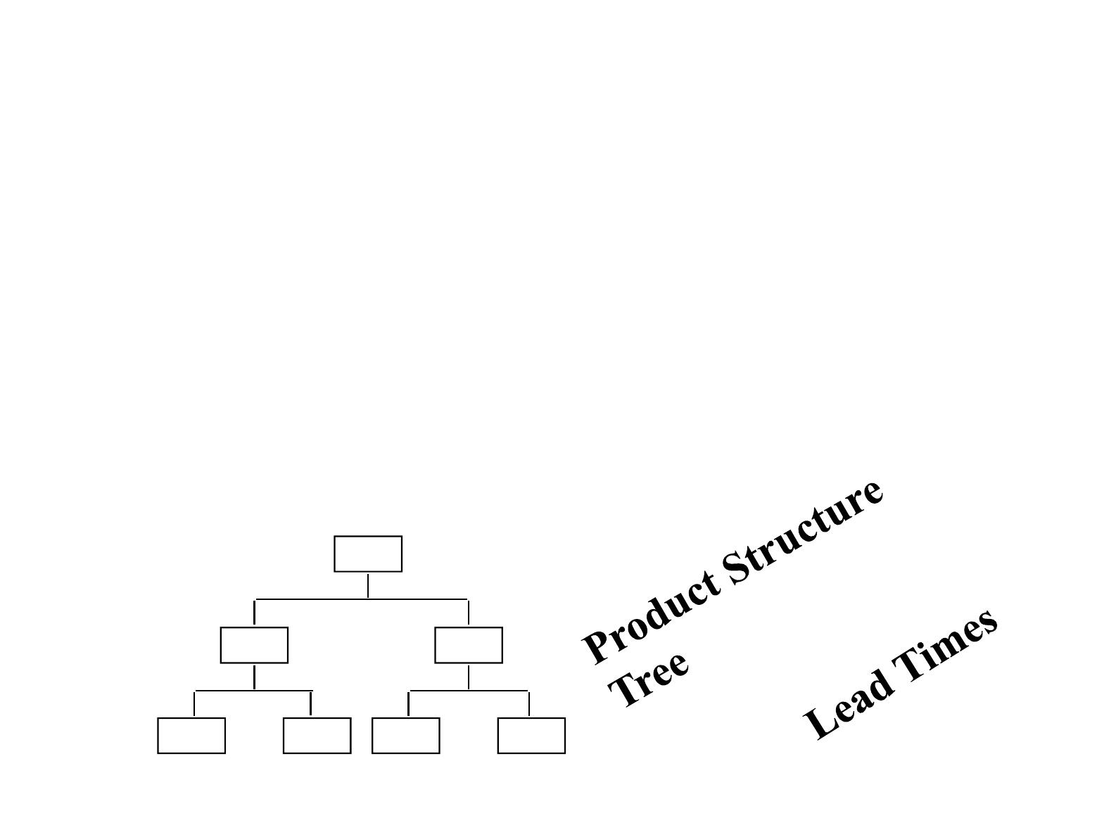
•Master Production Schedule
•Time-phased plan specifying timing and quantity of
MPR Inputs