Chapter
12
Inventory Management
DISCUSSION QUESTIONS
1. The short answer is that higher inventories do not provide an advantage in any of the nine
competitive priority categories. The important point is that firms must have the “right
amount” of inventory to meet their competitive priorities.
The only relevant costs considered in this chapter are ordering costs, holding costs,
and stockout costs. In the economic order quantity (EOQ) model, costs of placing
replenishment orders tradeoff against the costs of holding inventory. Under the
assumptions of the EOQ, average inventory is one-half of the order quantity. The number
of orders placed per year varies inversely with order quantity. When we consider
stockout costs, an additional inventory (safety stock), is held to trade-off costs of poor
customer service or costs for expediting shipments from unreliable suppliers.
In the lean systems chapter, we see order quantities (lot sizes) that are much smaller
than the “ideal” suggested by the EOQ model. As a result, lean systems average
inventory is also much lower. Are there some other relevant costs of holding inventory
that we have not considered in the EOQ model? If there are, a firm that ignores these
costs will make the wrong inventory decisions. These wrong decisions will make the firm
less competitive.
Let’s examine the relationships between inventory and the nine competitive priorities
discussed in the operations strategy chapter. We compare competitors H and L. They are
similar in all respects except H maintains much higher inventory than does L.
1) Low-cost operations. Costs include materials, scrap, labor, and equipment capacity
that are wasted when products are defective. When a process drifts out of control,
competitor H’s large lot sizes tend to result in large quantities of defectives. The EOQ
does not consider the cost of defectives, and erroneously assumes that setup costs are
constant. Small lots cause frequent setups, but the cost per setup decreases due to the
learning curve. Competitor L will enjoy competitive advantages with lower setup,
materials, labor, equipment, and inventory holding costs.
2) Top quality. Superior features, durability, safety, and convenience result from
improved designs. High inventories force competitor H to choose between scrapping
obsolete designs or delaying introduction of product improvements until the old
inventory is consumed. In either case, L gains a competitive advantage.
3) Consistent quality. Consistency in conforming to design specifications requires
consistency in supplied materials, setups, and processes. Small lots made frequently
tend to increase consistency. Again, advantage goes to L.
4) Delivery speed. Large lots take longer to produce than small lots. A customer will
wait less time for competitor L to set up and produce orders made in small batches.
Inventory Management • CHAPTER 12 • 307
5) On-time delivery. Contrary to expectations, large inventories do not equate to on-
time delivery. It’s more like, lots of inventory equals lots of chaos. Big lots make big
scheduling problems. Big lots get dropped, mishandled, and pilfered. Most lean
companies experience dramatic improvement in on-time delivery.
6) Development speed. This response is similar to that given for high-performance
design. Low inventories result in getting new designs to the market more quickly.
7) Customization. Lean companies usually don’t claim an advantage in customization.
However, large inventories provide no advantage with regard to customization either.
It remains unlikely that a customized product will be found in inventory, no matter
how large.
8) Variety. Mass customizers compete on service or product variety. They will keep
products at raw material or component levels until a customer orders a specific
configuration. Inventories are at as low a level as possible.
9) Volume flexibility. Lean (low inventory) companies tend to produce the same
quantity of every product every day, but they claim considerable volume flexibility
from month to month. On the other hand, a large finished goods inventory can be
used to absorb volume fluctuations.
In summary, a case can be made that several competitive priorities are not
considered in the EOQ model. It is sometimes difficult to place a dollar value on
these competitive advantages, but the advantages invariably go to the low-inventory,
small lot-size firm. So if the EQO is too large, what is the “ideal” lot size? According
to the lean philosophy, the “ideal” lot size is one.
2. Reducing cycle inventories has an effect on practically every functional area. Although
responses will vary, and sometimes be quite insightful, the following list contains some
standard answers:
Marketing—Reducing cycle inventories implies that there is less inventory on hand,
which could increase stockouts if the inventories are not managed properly.
Finance—Smaller-cycle inventories implies that there is less capital tied up in
inventory, thereby reducing the pressure for short-term operating capital and allowing for
alternative investment options.
Operations—Reducing cycle inventories implies that order quantities are to be
reduced. Order times and costs must be reduced to facilitate that move. Smaller order
quantities enable a shift toward a lean system and enhance a uniform flow of materials
through the production process.
3. Organizations will never get to the point where inventories are unneeded. Inventories
provide many functions and should be managed, not eliminated. It is impossible to
eliminate uncertainties in the provision of products or services. In addition, unless
materials can be transported instantaneously, there will always be pipeline inventories.
Cycle inventories will exist unless we universally get to the point where production of
single units is feasible.

308 • PART 3 • Managing Value Chains
PROBLEMS
1. A part
a. Average cycle inventory =Q2
==1000 2 500 units
Value of cycle inventory = (500 units) ($50+$60)
= $55,000
b. Pipeline inventory = dL
[(3800 units/year)/(50wks/yr)](6 weeks)
= 456 units
Value of the pipeline inventory = (456 units)($50+$30)
= $36,480
2. Prince Electronics
a. Value of each DC’s pipeline inventory
= (75 units/wk)(2 wk)($350/unit)
= $52,500
b. Total inventory = cycle + safety + pipeline
= 5[(400/2) + (2*75) + (2*75)]
= 2,500 units
3. Lockwood Industries
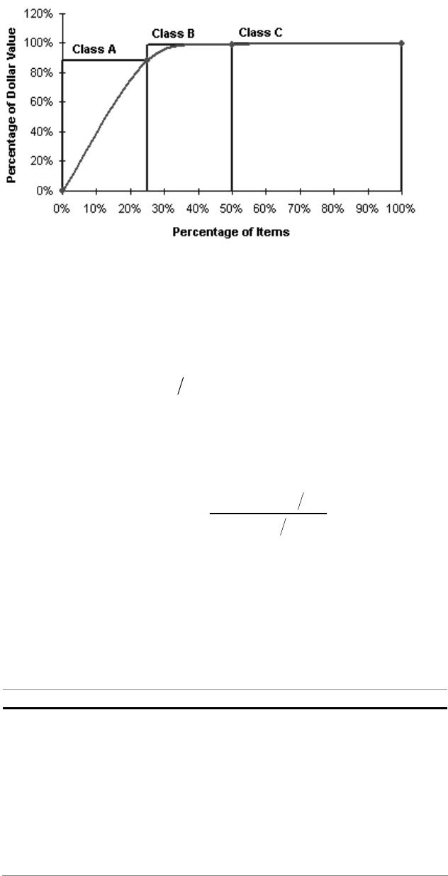
First we rank the items from top to bottom on the basis of their dollar usage. Then we
partition them into classes. The analysis was done using OM Explorer Tutor12.2—ABC
Analysis.
Cumulative % Cumulative %
Part # Description Qty Used/Yea
r
Value Dollar Usage Pct of Total of Dollar Value of Items Class
4 44,000 $1.00 $44,000 60.0% 60.0% 12.5% A
7 70,000 $0.30 $21,000 28.6% 88.7% 25.0% A
5 900 $4.50 $4,050 5.5% 94.2% 37.5% B
2 120,000 $0.03 $3,600 4.9% 99.1% 50.0% B
6 350 $0.90 $315 0.4% 99.5% 62.5% C
8 200 $1.50 $300 0.4% 99.9% 75.0% C
3 100 $0.45 $45 0.1% 100.0% 87.5% C
1 1,200 $0.01 $12 0.0% 100.0% 100.0% C
Total $73,322
Inventory Management • CHAPTER 12 • 309
The dollar usage percentages don’t exactly match the predictions of ABC analysis. For
example, Class A items account for 88.7% of the total, rather than 80%. Nonetheless, the
important finding is that ABC analysis did find the “significant few.” For the items
sampled, particularly close control is needed for items 4 and 7.
4. Terminator Inc.
a. Average cycle inventory =Q2
= 250/2
= 125 units
Value of cycle inventory = (125 units)($450)
= $56,250
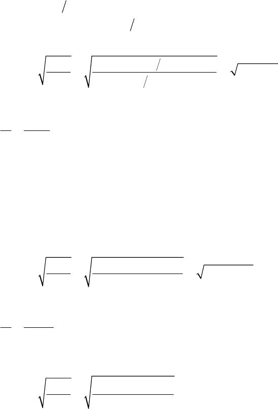
b. Pipeline inventory = dL
()
()
4,000 units yr 3 wk
50 wk yr
⎧⎫
=⎨⎬
⎩⎭
= 240 units
Value of pipeline inventory = (240 units)($150 + $300/2)
= $72,000
5. Stock-Rite Inc.
Computing the annual usage value for each item and rank ordering them highest to
lowest, we get:
Item Annual Value ($) Cumulative Value ($)
D205 9,690 9,690
U404 6,075 15,765 A: 55%
A104 3,220 18,985
L205 3,035 22,020 B: 22%
L104 2,005 24,025
S104 1,604 25,629
X205 1,603 27,232 C: 23%
X104 1,500 28,732
310 • PART 3 • Managing Value Chains
One classification might be to group the top two items (i.e., 25% of the items) in A class
accounting for 55% of the total value. The next two items would be classified as B and
the last four as C.
The dollar usage percentages don’t exactly match the predictions of ABC analysis.
For example, Class A items account for only 55% of the total, rather than 80%.
Nonetheless, the important finding is that ABC analysis did find the “significant few.”
For the items sampled, particularly close inventory management is needed for items
D205 and U404.
6. Yellow Press, Inc.
a. Economic order quantity
()
()()
2500 rolls
Price $800 roll
15% $800 $120 roll-year
$50
2 2 2500 rolls year $50 2083.33 45.64 or 46 rolls
$120 roll-year
D
H
S
DS
EOQ H
=
=
==
=
== = =
b. Time between orders
46 0.0184 year, or every 4.6 days
2500
if there are 250 working days in a year
==
Q
D
7. Babble Inc.
a. 400d= tapes/month
4800D= tapes/year
$0.12
$12.50
H
S
=
=
()( )
2 2 4,800 $12.50 1,000,000 1000 tapes
$0.12
DS
EOQ H
== = =
b. Time between orders
1, 000 0.2083
4,800
Q
D== years or 2.5 months
8. Dot Com
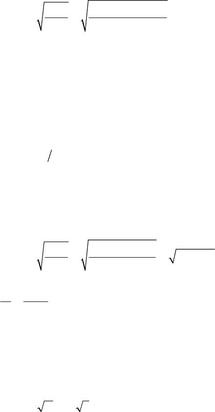
a.
()()
2 32,000 $10
2400 books
$4
DS
EOQ H
== =
b. Optimal number of orders/year = (32,000)/400 = 80 orders
c. Optimal interval between orders = 300/80 = 3.75 days
d. Demand during lead time = dL = (5 days)(32,000/300) = 533 books
Inventory Management • CHAPTER 12 • 311
e. Reorder point = dL + safety stock = 533 + 0 = 533 books
f. Inventory position = OH + SR – BO = 533 + 400 – 0 = 933 books
9. Leaky Pipe Inc.
a.
()()
2 30,000 $10
2775 units
$1
DS
EOQ H
== =
b. Optimal number of orders = (30,000)/(775) = 38.7 or 39
c. Optimal interval between orders = (300)/(39) = 7.69 days
d. Demand during lead time = dL = (4 days)(30,000/300) = 400 units
e. Reorder point = dL + safety stock = 400 + 0 = 400 units
f. Inventory position = OH + SR – BO = 400 +775 – 0 = 1175 units
10. Sam’s Cat Hotel
a. Economic order quantity
()
()()
90 week
4,680
$54
Price $11.70
27% $11.70 $3.159
2 4,680 54
2160,000 400 bags
3.159
d
D
S
H
DS
EOQ H
=
=
=
=
==
== = =
Time between orders, in weeks
Q
D== =
400
4680 0 08547 4 44.. years weeks
b. Reorder point, R
R = demand during protection interval + safety stock
Demand during protection interval = dL = 90 * 3 = 270 bags
Safety stock =zL
σ
When the desired cycle-service level is 80%, z=084..
σσ
Lt
L===15 3 26 = 25.98 or 26
Safety stock = 0.84 * 26 = 21.82 or about 22 bags
R
=+=270 22 292
c. Initial inventory position = OH + SR – BO = 320 + 0 – 0
320 – 10 = 310.
Because inventory position remains above 292, it is not yet time to place an order.
312 • PART 3 • Managing Value Chains
d. Annual holding cost Annual ordering cost
QH
2
500
227% 70
75
=()( )
=
$11.
$789.
4,680 $54
500
$505.44
=
=
DS
Q
At the EOQ, these two costs are equal. When Q=500 , the annual holding cost is
larger than the ordering cost, therefore Q is too large. Total costs are $789.75 +
$505.44 = $1,295.19.
e. Annual holding cost Annual ordering cost
QH
2
400
227% 70
80
=()( )
=
$11.
$631.
4,680 $54
400
$631.80
DS
Q=
=
Total costs at EOQ: = $1,263.60, which is $31.59 less than when order quantity is
500 bags.
11. Sam’s Cat Hotel, revisited
a. If the demand is only 60 bags per week, the correct EOQ is: