Monte Carlo simulation: The Atomic bomb your project doesn’t need
Ivan Arturo Traverso
Monte Carlo technique was developed by Stanislaw Ulam and John von Neuman during
the World War II. It helped to develop the atomic Bomb while solving issues related to diffusion
of neutrons during fission. Nowadays, Monte Carlo has spread into many researches and
applications on diverse fields. There are several financial planning softwares that apply Monte
Carlo simulation analysis. A complex technique that relies on thousands of random simulations
surely impresses and attains trust about the result deducted by the simulation. But, is this
technique really trustworthy in real market decisions? How much can the assumptions generally
made by analysts when developing a Monte Carlo simulation really affect the results? Jhon D,
Kingston, Principal of a registered investment advisor company in the U.S.A indicates “The
benefit that Monte Carlo simulation promises to provide might be better achieved by using
common sense in the financial planning process” (2001, p.104).
When a variable is modeled in Monte Carlo’s framework, it is reduced to several
assumptions. Most of the times, the relation between each variable is overlooked and they are
treated simply as random independent variables. Even if not, modeling variables considering all
the relations between variables could result an unaffordable task. Phd Finance Professor David
Nawrocki (2001), explain the three principal kinds of relations between variables and how
problematic is each of them for Monte Carlo’s modeling:
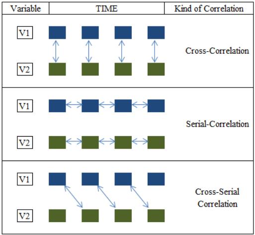
1. Cross Correlation, that is the dependence of each possible result of one variable
affecting directly the other. This kind of relationship is still relatively not difficult to be
modeled on a Monte Carlo spreadsheet.
2
2. Serial Correlation, It happens when each result affects the consequents of the same
variable. When the variable results have significant dependence over the time,
formulating properly it on a model could result problematic.
3. Cross-Serial Correlation, this is stated if each possible value affects over the time the
next results of the second variable. At this point, modeling a variable for a Monte Carlo
simulation is extremely complex.
According to Nawrocki, An example of variables with all three relationships is possible
to be found between Nasdaq 100 Index and S&P 500 index, both important stock market indexes
in the U.S. (2001). Figure 1 resumes graphically the three main kinds of correlation between
variables. Moreover, if it is considered that real life relations between variables adopt complex
interactions between many of them on very large periods of time, conducting a Monte Carlo
simulation could result a very time consuming task with low trustworthiness.
Figure 1. Kinds of Correlation between Variables

3
To complicate things further, some empirical work such as the developed by Whitelaw
(1994), and Perez-Quiroz & Timmermann (2000), indicate that means and standard deviations
vary through along a business cycle. Calculating and then introducing the variability on those
statistical elements of a Monte Carlo simulation surely require an intricate study. That is why
most analysts just assume that markets are explained by just one mean and one standard
deviation in normal distributions. They should at least contemplate the significances of not
taking into account the non-stationary distributions into the Monte Carlo simulation model.
Starting to consider Monte Carlo simulation a courageous project? Well, there is one
more consideration to fit into the very complex simulation: Non-linear Relationships of