Discussion Questions
1. What forecasting method would fulfill the company’s specifications? Please justify.
2. What is the forecast of aggregate demand by month for the year 2012?
3. In addition to forecasting demand of larger customers and aggregate demand, how might
the accuracy of the forecast be improved?
4. What role should Ed Merriwell’s feel of the market play in establishing new sales
forecasts?
Merriwell Bag Company manufactures and distributes stock bags to many small chain
stores scattered over a wide geographical area. Presently, due to growth in the business,
forecasting demand has become more difficult. As a result, the company would like a
forecasting system developed. Monthly data from the past five years is provided in the
case.
This case presents an opportunity for the student to design a forecasting system. The case
also asks the student to describe how the system can be used and aided by managerial
judgment.
Analysis
Because of the seasonal nature of the demand facing Merriwell Bag Company, an
appropriate forecasting tool is the classical decomposition method (discussed in the
supplement to Chapter 11). The data in the case is provided on the website for the
textbook. Only the data is provided on the Excel template from the website. The user must
enter the formulas and analysis.
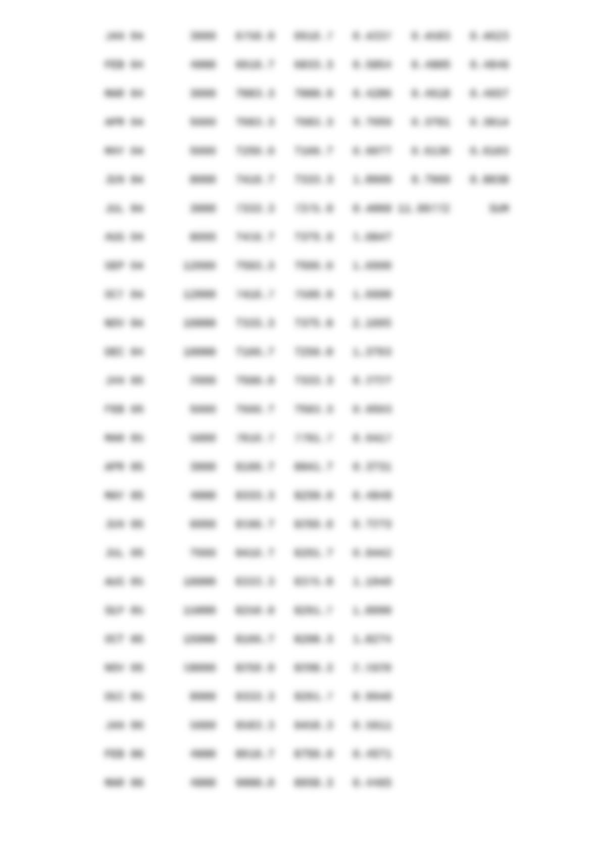
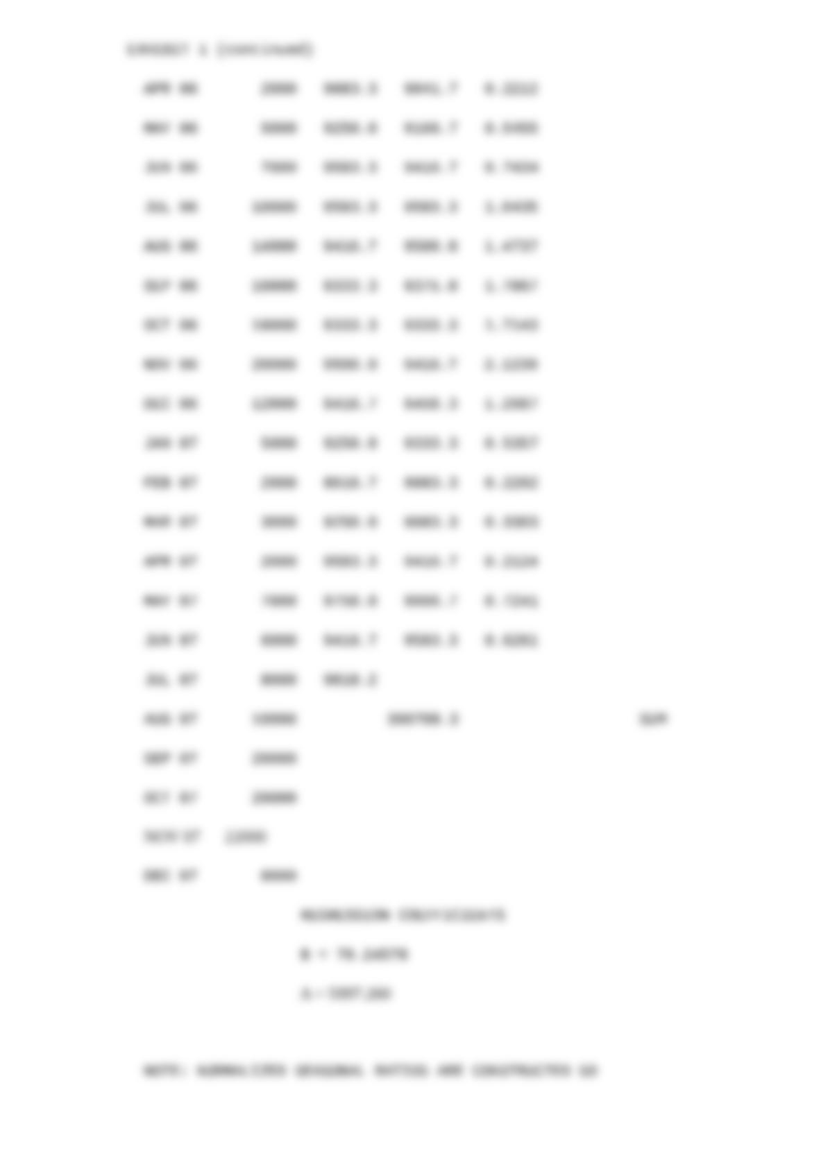
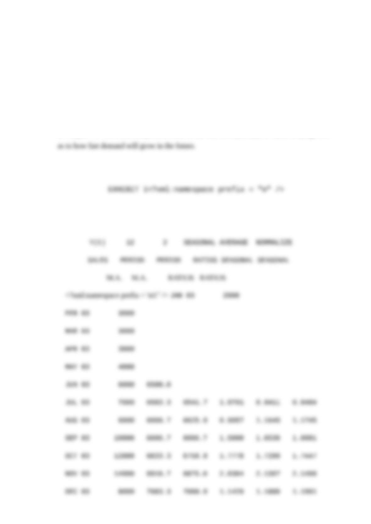
Sixty months of data are provided on the template, see Exhibit 1. The first step in classical
decomposition is to develop a 12-month moving average which is done in the 3rd column
on the worksheet. Then a 2-month moving average is developed in the 4th column which
is centered on the original data. The 4th column contains data which is deseasonalized,
since 12 months has been used as a base in the moving average. At this point the upward
trend in the moving average in column 4 is apparent.
In column 5 seasonal ratios are computed by dividing the sales data for each month by the
moving average in column 4. The data indicates that high seasonal demand occurs before
Christmas each year in September, October and November. Low seasonal demand occurs
in the January, February, and March time frame. In column 6 average seasonal ratios are
computed. These ratios are obtained by averaging the seasonal ratios from the same month
in successive years. For example, the July 2011 seasonal ratio is obtained by averaging the
July 2007, July 2008, July 2009, and July 2010 seasonal ratios.
When the resulting twelve seasonal ratios are added the total is 11.8977. The sum of these
ratios should be 12 in accordance with the 12-month seasonal period, because the seasonal
ratio is the percentage that a particular month is above or below the average. In order to
obtain a sum of 12, the seasonal ratios are normalized in column 7. This is done by
dividing each ratio by the sum 11.8977 and multiplying by 12.
A regression analysis is now run to fit a straight line through the moving average data in
column 4. The purpose of this regression is to forecast the average level into 2008 on a
trend basis. The seasonal ratios will then be applied to this trend to arrive at a forecast. In
Excel a regression function is provided. In this case we have data from period 7 through
period 54. The formulas and procedure for calculating the regression equation are given in
the text. As a result of these calculations the following equation is obtained.
Y = 5997 + 70.24 t
Where Y is the moving average and t is the time period.
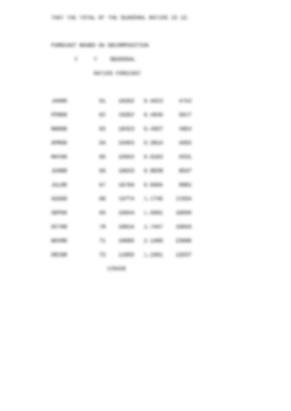
To obtain the forecast of interest we calculate Y from the above equation for the twelve
months of 2012, which is t = 61 through t = 72. These Y values are multiplied by the
monthly average seasonal ratios to arrive at the forecast for each month shown in Exhibit
1. Note that the total of this forecast is 129,435 bales of bags for the year 2012.
In evaluating the forecast one of the questions that comes to mind is the validity of the
linear trend assumption. Note, that total demand in 2011 (113,000) was actually a little less
than the total demand for 2010 (115,000). Ed Merriwell should determine if there is some
reason for this leveling out of demand or should the historical trend be assumed to resume.
If demand flattens out at 115,000 bales, our forecast for 2012 could be too high by about
15,000 bales for the year (129,435 – 115,000).
The seasonal ratios appear to be pretty stable from year to year. While some monthly
variation can be expected in seasonal ratios, it will probably not be as serious as the trend
assumption discussed above, because the seasonal error from month to month will tend to
average out over the course of 2012.
Whereas the above forecasting technique should be useful, Ed Merriwell’s “feel” of the
market should not be discarded. Any analytical method should be augmented by personal
judgment. This judgment would prove very useful in considering mostly non-quantifiable
factors that might affect demand (state of the economy, consumer attitudes, activity of
competitors, etc.) These effects can be quantitatively introduced into the forecast by
adjusting the future trend and possibly the individual seasonal ratios.
This case can also be analyzed by using exponential smoothing with seasonal adjustments
and trend. A spreadsheet could be written using the Winter’s formulas from the supplement
to Chapter 11. The trend component could be derived from past data or based on judgment