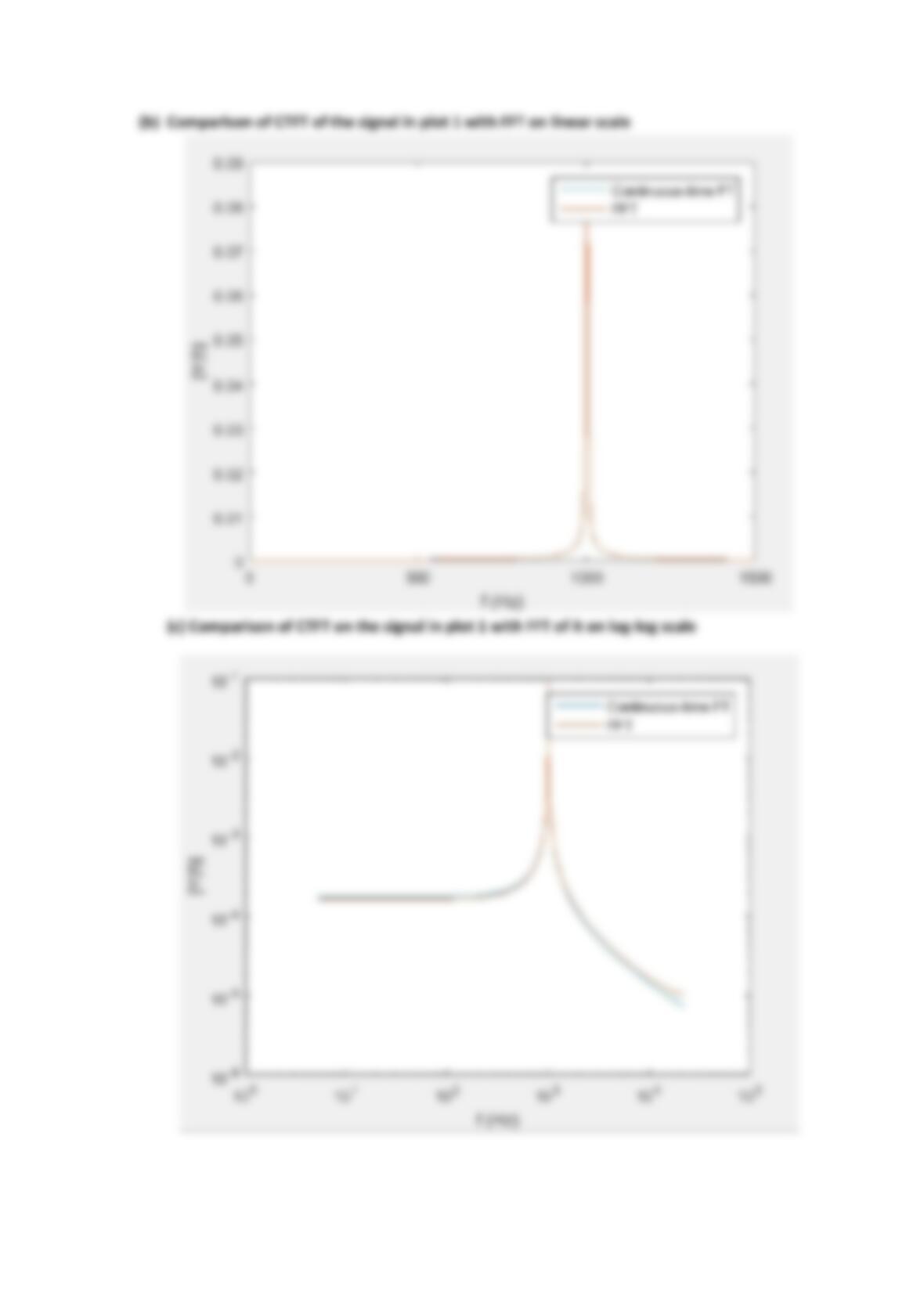
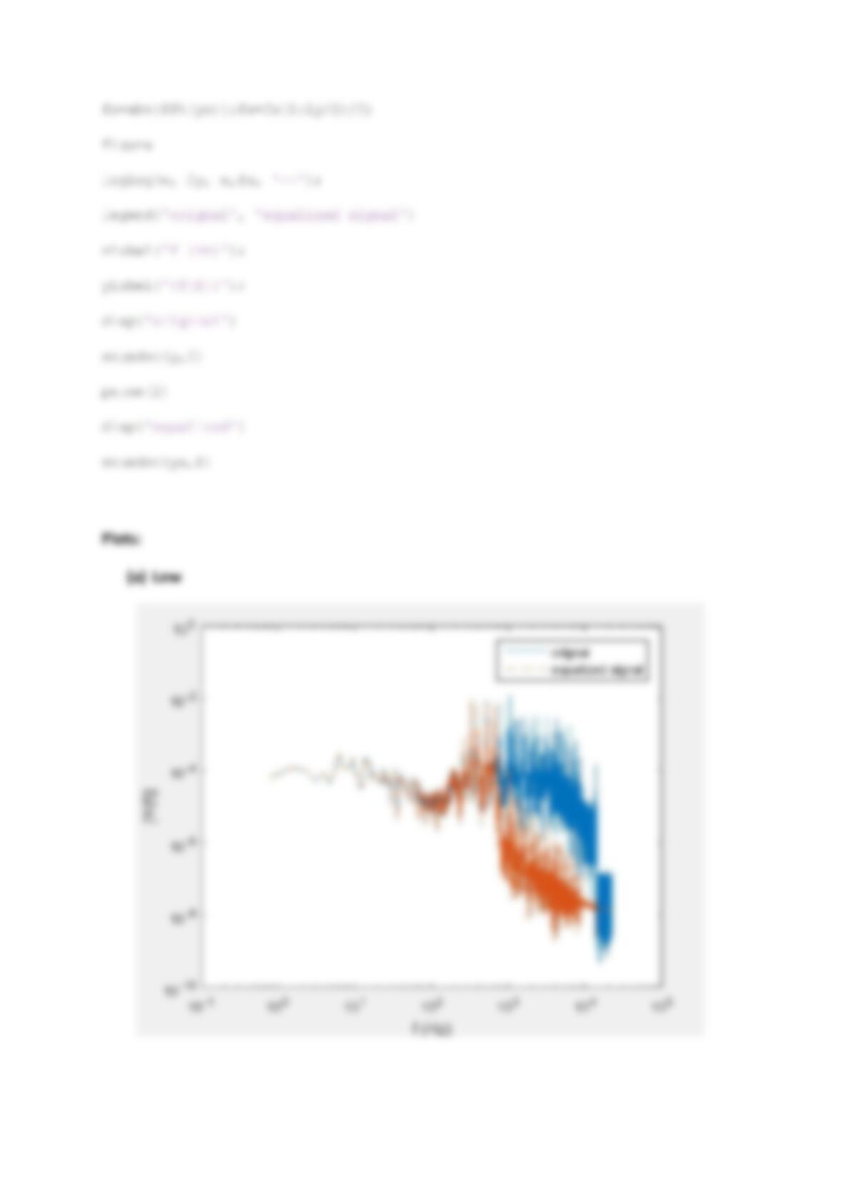
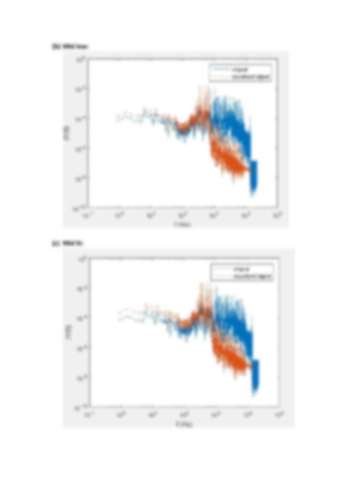
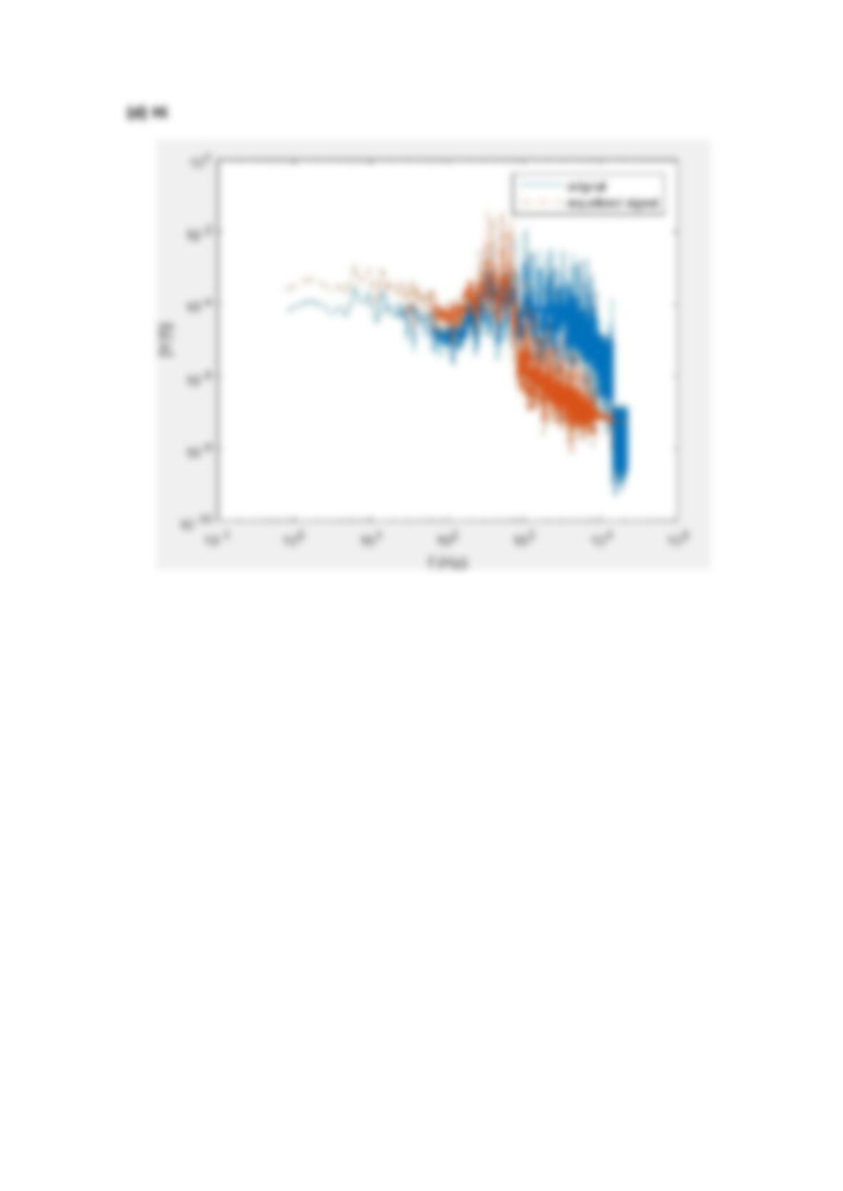
Lab Description
In this lab we have implemented sampling theory to different audio signals and analyzed the
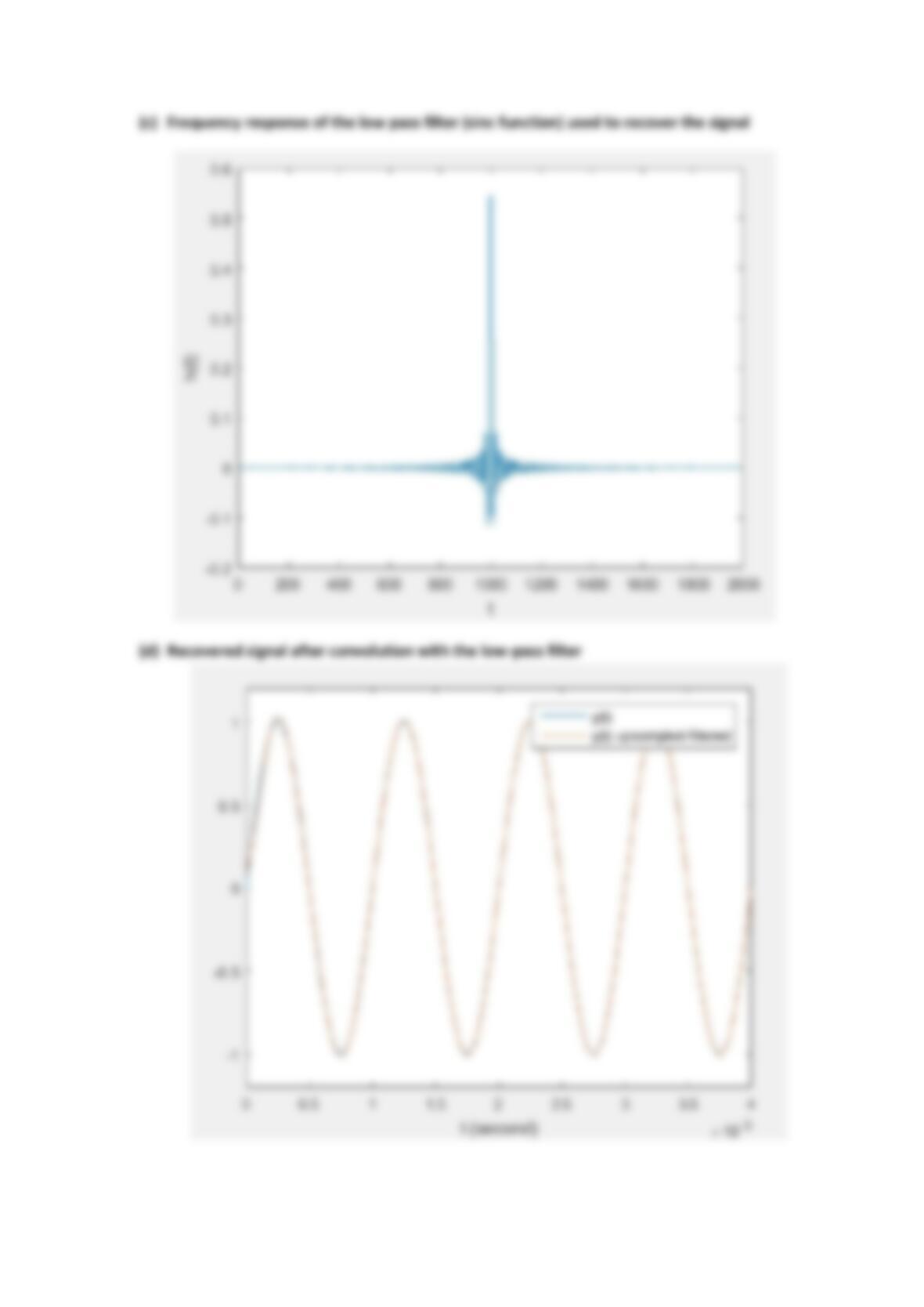
responses. We have understood zero order hold. The zero-order hold (ZOH) is a mathematical model
of the practical signal reconstruction done by a conventional digital-to-analogue converter (DAC).
That is, it describes the effect of converting a discrete-time signal to a continuous-time signal by
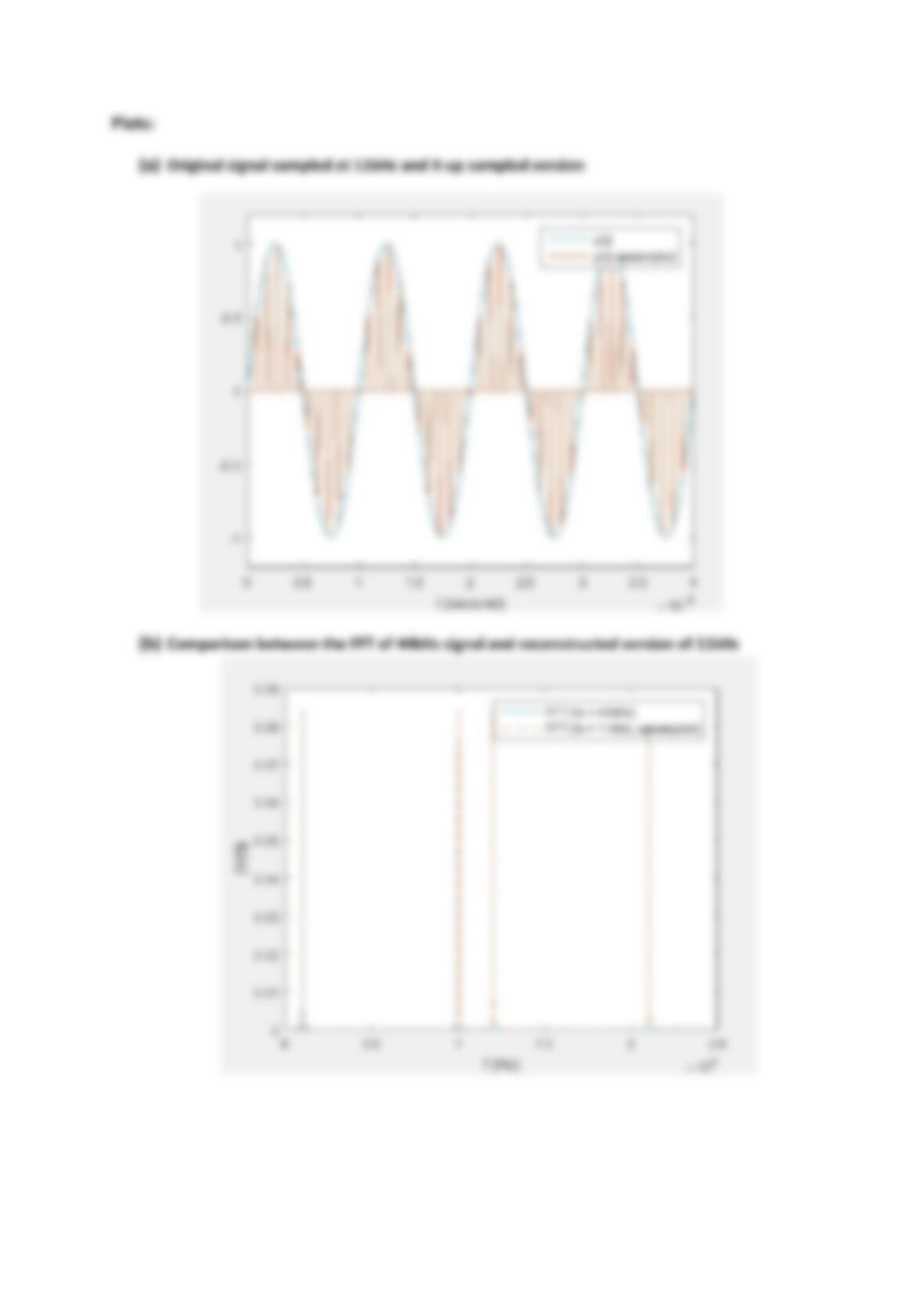
holding each sample value for one sample interval. We have analysed the sound signals and beep
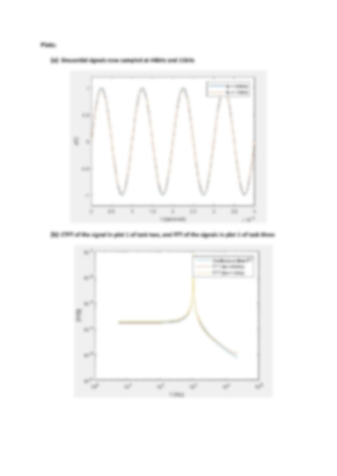
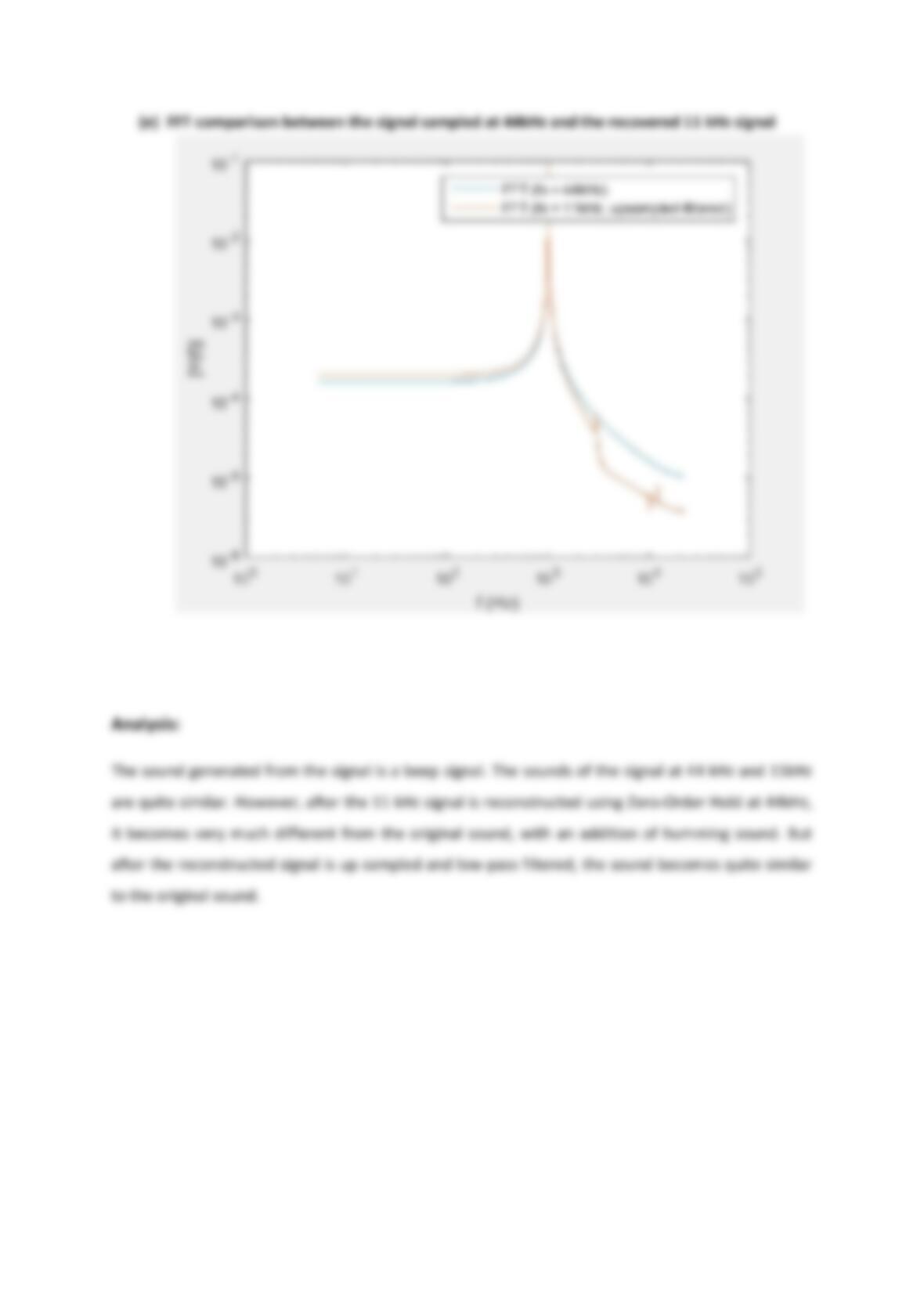
signals. The sounds of the signal at 44 kHz and 11kHz are quite similar. However, after the 11 kHz
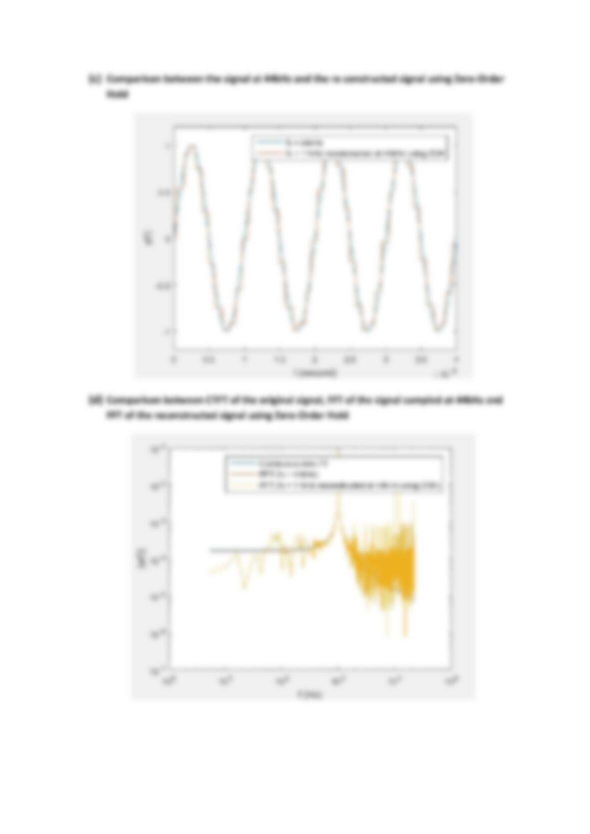
signal is reconstructed using Zero-Order Hold at 44kHz, it becomes very much different from the
original sound, with an addition of humming sound. But after the reconstructed signal is up sampled
and low-pass filtered, the sound becomes quite similar to the original sound.
Task 1:
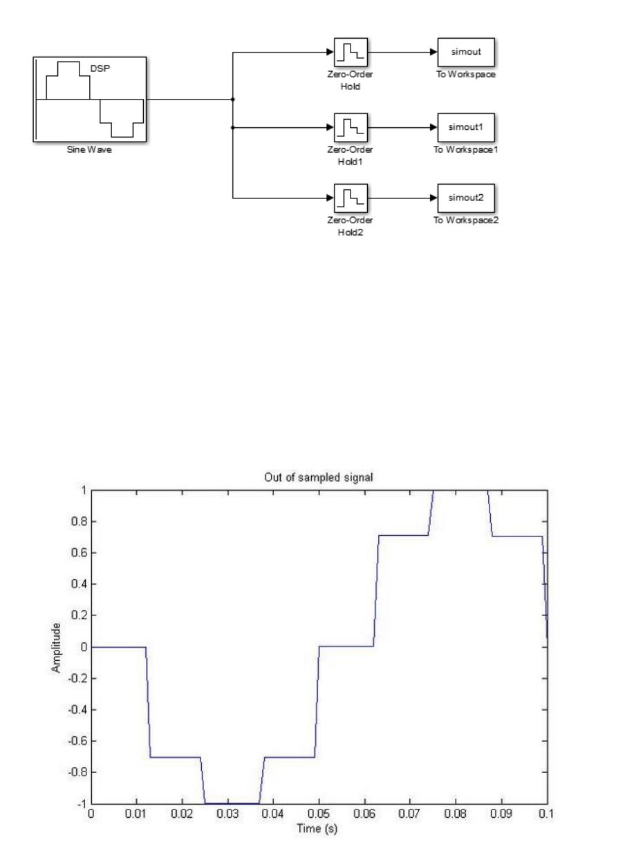
Simulink model:
Plots:
(a) Plot of output with sampling frequency 80 Hz
Data = simout.signals.values;
Time = simout.time;
plot (Data,Time)
title(‘Out of sampled signal’)
xlabel (‘Time(s)’)
ylabel (‘Amplitude’)
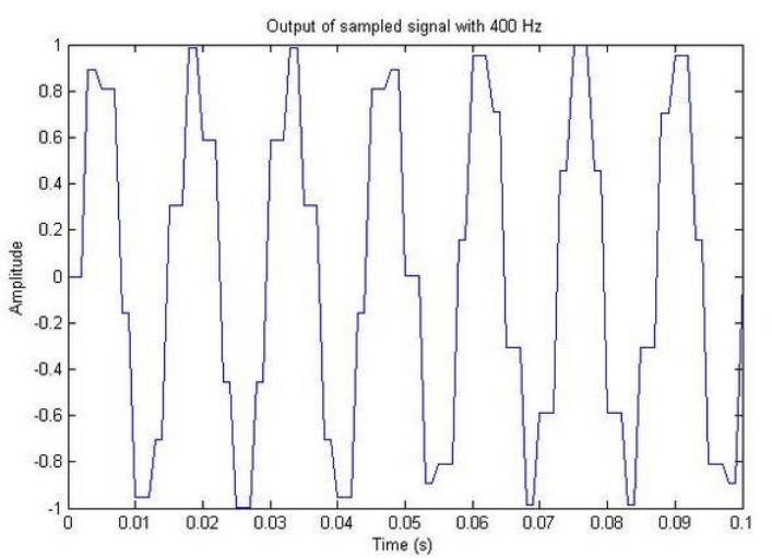
(b) Plot of output with sampling frequency of 400 Hz
Data1 = simout1.signals.values
Time1 = simout1.time
plot (Data1,Time1)
title(‘Output of sampled signal with 400Hz’)
xlabel (‘Time(s)’)
ylabel (‘Amplitude’)
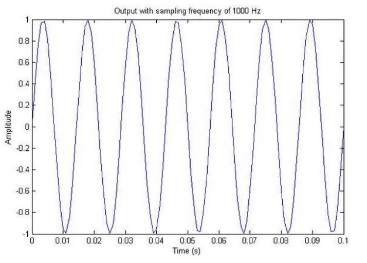
(c) Plot of output with sampling frequency 1000 Hz
Data2 = simout2.signals.values
Time2 = simout2.time
plot (Data1,Time1)
title(‘Output of sampled signal with 1000Hz’)
xlabel (‘Time(s)’)
ylabel (‘Amplitude’)
Task 2:
Matlab Code:
close all;
clear all;
% plot the time domain signal
% Define the sampling frequency and the time vector. (8000 points / 44 kHz
~ 0.2 s worth of data)
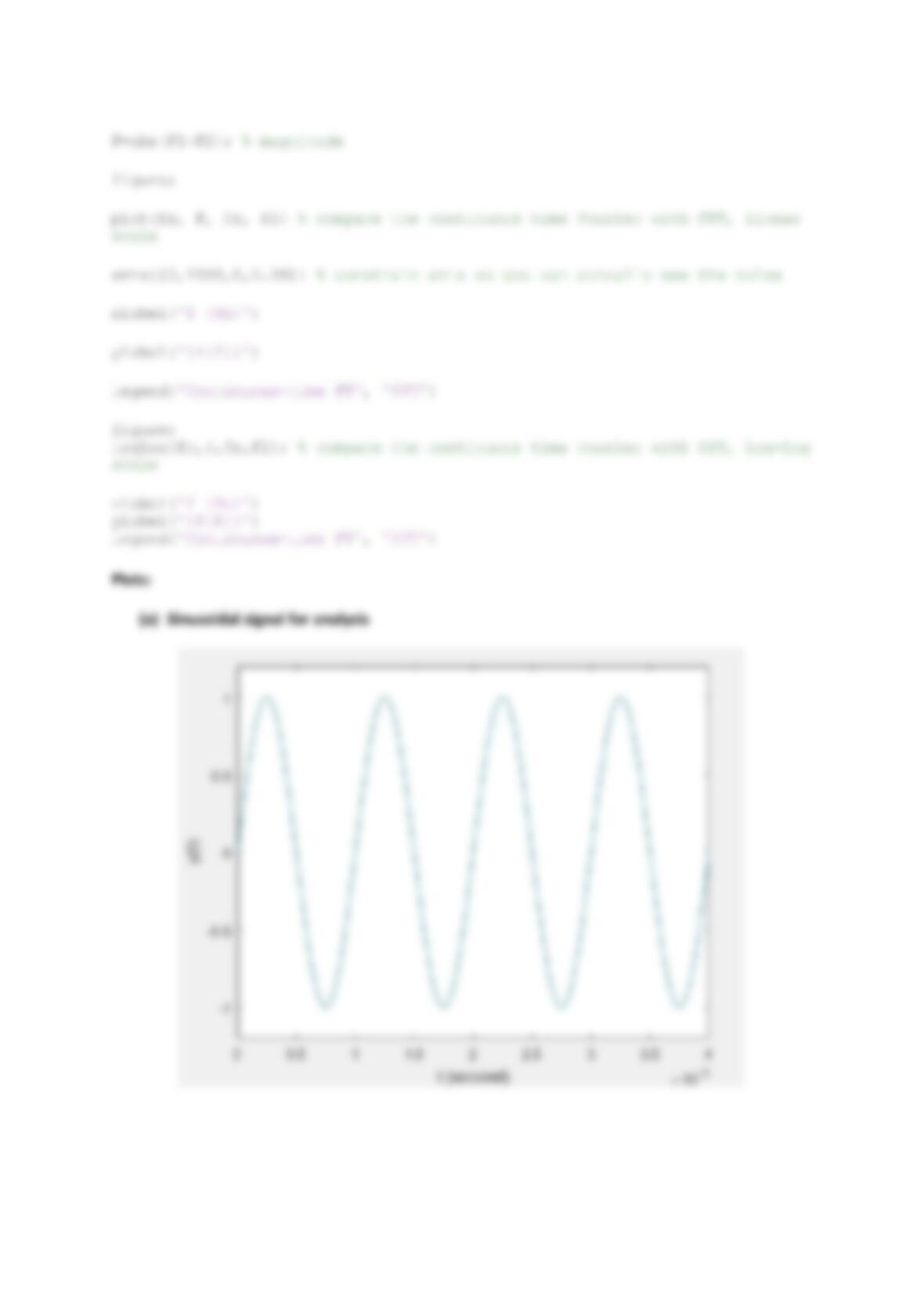
% Plot the output and look at the first 0.004s.
fs=44100; no_pts=8192;
t=([0:no_pts-1]’)/fs;
y1=sin(2*pi*1000*t);
figure;
plot(t,y1);
xlabel(‘t (second)’)
ylabel(‘y(t)’)
axis([0,.004,-1.2,1.2]) % constrain axis so you can actually see the wave