Linear Equation Method and Graphical Presentation
Demand Curve
Demand is the economic principle which shows the consumer’s willingness to purchase goods
and services, and to pay price for the goods. So, an increase in the prices will negatively affect
the quantity demanded while keeping other factors constant.
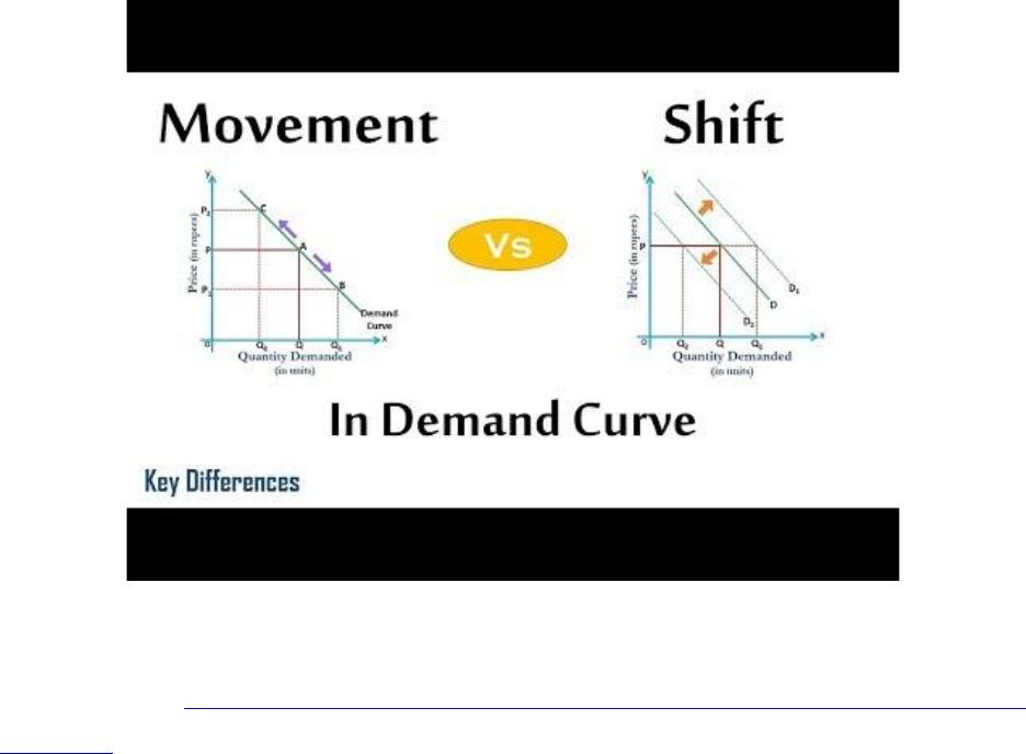
Figure 1: Demand Curve
Source: https://keydifferences.com/difference-between-movement-and-shift-in-demand-
curve.html
Firstly, demand curve is the graphical representation which shows the relationship between the
price and quantity demanded of a good for a certain time period as shown the above diagram.
There is an inverse relationship between the price and quantity demanded also known as law of
demand. As other factors remain constant includes consumer behavior, number of customers in
market, income and substitute goods prices, known as the ceteris paribus which cause the
movement along the demand curve moving from point A to B to C or vice versa as shown in
diagram. Whereas if these factors change which will cause the demand curve to shift inward or
outwards (Gans, King & Mankiw, 2011). Secondly, demand curve can also be derived from the
linear equation method. It shows the quantity demanded (Qd) as the function of the price (P).
The linear demand equation is Qd=a+Pm and demand curve can be plotted using this equation by
plugging in values. Where “a” indicates all factors that affects price other than the factors like
mentioned above and “m” is the slope of demand curve. Moreover, finding the ordered price and
function the calculate the slope and its y-intercept (Qd is zero), these values will help plot the
curve.
Supply Curve