© 2012 Pearson Education, Inc. Publishing as Prentice Hall
Chapter 13
Leverage and Capital Structure
Answers to Warm-Up Exercises
E13-1. Breakeven analysis
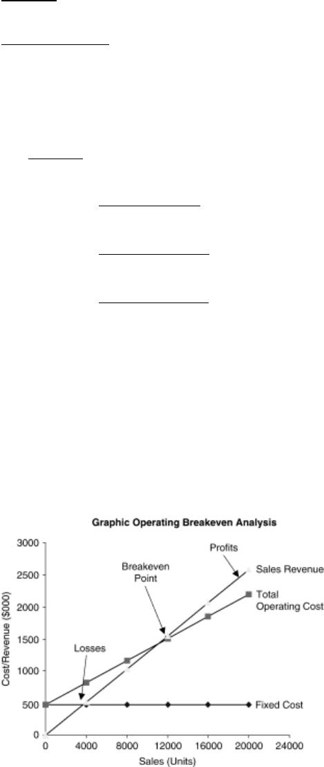
Answer: The operating breakeven point is the level of sales at which all fixed and variable operating
costs are covered and EBIT is equal to $0.
Q FC (P – VC)
Q $12,500 ($25 $10) 833.33, or 834 units
E13-2. Changing costs and the operating breakeven point
Answer: Calculate the breakeven point for the current process and the breakeven point for the new
process, and compare the two.
Current breakeven: Q1 $15,000 ($6.00 $2.50) 4,286 boxes
New breakeven: Q2 $16,500 ($6.50 $2.50) 4,125 boxes
If Great Fish Taco Corporation makes the investment, it can lower its breakeven point by
161 boxes.
E13-3. Risk-adjusted discount rates
Answer: Use Equation 13.5 to find the DOL at 15,000 units.
15,000
$20
$12
$30,000
Q
P
VC
FC
15,000 ($20 $12) $120,000
DOL at 15,000 units 1.33
15,000 ($20 $12) $30,000 $90,000
E13-4. DFL
Answer: Substitute EBIT $20,000, I $3,000, PD $4,000, and the tax rate (T 0.38) into
Equation 12.7.
$20,000
DFL at $20,000 EBIT $20,000 $3,000 [$4,000 (1 (1 0.38)]
$20,000 1.90
$10,548
E13-5. Net operating profits after taxes (NOPAT)
Answer: Calculate EBIT, then NOPAT and the weighted average cost of capital (WACC) for Cobalt
Industries.
EBIT (150,000 $10) $250,000 (150,000 $5) $500,000
NOPAT EBIT (1 T) $500,000 (1 0.38) $310,000
NOPAT $310,000
Value of the firm $3,647,059
0.085
a
r
Solutions to Problems
P13-1. Breakeven point—algebraic
LG1; Basic
()
$12,350 1,300
($24.95 $15.45)
FC
QP VC
Q
P13-2. Breakeven comparisons—algebraic
LG 1; Basic
a.
()
FC
QP VC
Firm F:
$45,000 4,000 units
$18.00 $6.75
Q
Firm G:
$30,000 4,000 units
$21.00 $13.50
Q
Firm H:
$90,000 5,000 units
$30.00 $12.00
Q
b. From least risky to most risky: F and G are of equal risk, then H. It is important to recognize
that operating leverage is only one measure of risk.
P13-3. Breakeven point—algebraic and graphical
LG 1; Intermediate
a. Q FC (P VC)
Q $473,000 ($129 $86)
Q 11,000 units
b.
P13-4. Breakeven analysis
LG 1; Intermediate

a.
$73,500 21,000 CDs
$13.98 $10.48
Q
b. Total operating costs FC (Q VC)
Total operating costs $73,500 (21,000 $10.48)
Total operating costs $293,580
c. 2,000 12 24,000 CDs per year. 2,000 records per month exceeds the operating breakeven
by 3,000 records per year. Barry should go into the CD business.
d. EBIT (P Q) FC (VC Q)
EBIT ($13.98 24,000) $73,500 ($10.48 24,000)
EBIT $335,520 $73,500 $251,520
EBIT $10,500
P13-5. Personal finance: Breakeven analysis
LG 1; Easy
a. Breakeven point in months fixed cost ÷ (monthly benefit – monthly variable costs)
$500 ($35 $20) $500 $15 33 1/3 months
b. Install the Geo-Tracker because the device pays for itself over 33.3 months, which is less than
the 36 months that Paul is planning on owning the car.
P13-6. Breakeven point—changing costs/revenues
LG 1; Intermediate
a. Q F (P VC) Q $40,000 ($10 $8) 20,000 books
b. Q $44,000 $2.00 22,000 books
c. Q $40,000 $2.50 16,000 books
d. Q $40,000 $1.50 26,667 books
e. The operating breakeven point is directly related to fixed and variable costs and inversely
related to selling price. Increases in costs raise the operating breakeven point, while increases
in price lower it.
P13-7. Breakeven analysis
LG 1; Challenge
a.
$4,000 2,000 figurines
( ) $8.00 $6.00
FC
QP VC
b. Sales $10,000
Less:
Fixed costs 4,000
Variable costs ($6 1,500) 9,000
EBIT $3,000
c. Sales $15,000
Less:
Fixed costs 4,000
Variable costs ($6 1,500) 9,000
EBIT $2,000
d.
EBIT $4,000 $4,000 $8,000 4,000 units
$8 $6 $2
FC
QP VC

e. One alternative is to price the units differently based on the variable cost of the unit. Those
more costly to produce will have higher prices than the less expensive production models. If
they wish to maintain the same price for all units they may need to reduce the selection from
the 15 types currently available to a smaller number that includes only those that have an
average variable cost below $5.33 ($8 $4,000/1,500 units).
P13-8. EBIT sensitivity
LG 2; Intermediate
a. and b.
8,000 Units
10,000 Units
12,000 Units
Sales
$72,000
$90,000
$108,000
Less: Variable costs
40,000
50,000
60,000
Less: Fixed costs
20,000
20,000
20,000
EBIT
$12,000
$20,000
$ 28,000
c.
Unit Sales
8,000
10,000
12,000
Percentage
(8,000 10,000) 10,000
(12,000 10,000) 10,000
Change in
unit sales
20%
0
20%
Percentage
(12,000 20,000) 20,000
(28,000 20,000) 20,000
Change in
EBIT
40%
0
40%
d. EBIT is more sensitive to changing sales levels; it increases/decreases twice as much as sales.
P13-9. DOL
LG 2; Intermediate
a.
$380,000 8,000 units
( ) $63.50 $16.00
FC
QP VC
9,000 Units
10,000 Units
11,000 Units
b.
Sales
$571,500
$635,000
$698,500
Less: Variable costs
144,000
160,000
176,000
Less: Fixed costs
380,000
380,000
380,000
EBIT
$ 47,500
$ 95,000
$142,500
c.
Change in unit sales
1,000
0
1,000
% change in sales
1,000 10,000
10%
0
1,000 10,000 10%
Change in EBIT
$47,500
0
$47,500
% Change in EBIT
$47,500 95,000 = 50%
0
$47,500 95,000 =
50%
d.
% change in EBIT
% change in sales
50 10 5
50 10 5
e.
[ ( )]
DOL [ ( )]
Q P VC
Q P VC FC
[10,000 ($63.50 $16.00)]
DOL [10,000 ($63.50 $16.00) $380,000]
$475,000
DOL 5.00
$95,000
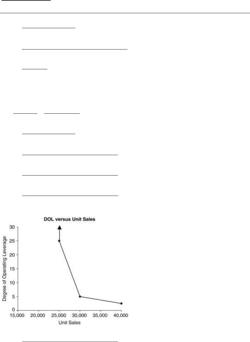
P13-10. DOL—graphic
LG 2; Intermediate
a.
$72,000 24,000 units
( ) $9.75 $6.75
FC
QP VC
b.
[ ( )]
DOL [ ( )]
Q P VC
Q P VC FC
[25,000 ($9.75 $6.75)]
DOL 25.0
[25,000 ($9.75 $6.75)] $72,000
[30,000 ($9.75 $6.75)]
DOL 5.0
[30,000 ($9.75 $6.75)] $72,000
[40,000 ($9.75 $6.75)]
DOL 2.5
[40,000 ($9.75 $6.75)] $72,000
c.
d.
[24,000 ($9.75 $6.75)]
DOL [24,000 ($9.75 $6.75)] $72,000
At the operating breakeven point, the DOL is infinite.
e. DOL decreases as the firm expands beyond the operating breakeven point.

P13-11. EPS calculations
LG 2; Intermediate
(a)
(b)
(c)
EBIT
$24,600
$30,600
$35,000
Less: Interest
9,600
9,600
9,600
Net profits before taxes
$15,000
$21,000
$25,400
Less: Taxes
6,000
8,400
10,160
Net profit after taxes
$ 9,000
$12,600
$15,240
Less: Preferred dividends
7,500
7,500
7,500
Earnings available to
common shareholders
$ 1,500
$ 5,100
$ 7,740
EPS (4,000 shares)
$ 0.375
$ 1.275
$ 1.935
P13-12. Degree of financial leverage
LG 2; Intermediate
a.
EBIT
$80,000
$120,000
Less: Interest
40,000
40,000
Net profits before taxes
$40,000
$ 80,000
Less: Taxes (40%)
16,000
32,000
Net profit after taxes
$24,000
$ 48,000
EPS (2,000 shares)
$ 12.00
$ 24.00
b.
EBIT
DFL 1
EBIT (1 )
I PD T
$80,000
DFL 2
[$80,000 $40,000 0]
c.
EBIT
$80,000
$120,000
Less: Interest
16,000
16,000
Net profits before taxes
$64,000
$104,000
Less: Taxes (40%)
25,600
41,600
Net profit after taxes
$38,400
$ 62,400
EPS (3,000 shares)
$ 12.80
$ 20.80
$80,000
DFL 1.25
[$80,000 $16,000 0]
P13-13. Personal finance: Financial leverage
LG 2; Challenge
a.
Current DFL
Initial Values
Future Value
Percentage
Change
Available for making loan payment
Less: Loan payments
Available after loan payments
$3,000
$1,000
$2,000
$3,300
$1,000
$2,300
10.0%
0.0%
15.0%
DFL
15% ÷ 10% 1.50
Proposed DFL
Initial Values
Future Value
Percentage
Change
Available for making loan payment
Less: Loan payments
Available after loan payments
$3,000
$1,350
$1,650
$3,300
$1,350
$1,950
10.0%
0.0%
18.2%
DFL
18.2% ÷ 10% 1.82
b. Based on his calculations, the amount that Max will have available after loan payments with
his current debt changes by 1.5% for every 1% change in the amount he will have available