1
1
Chapter 5 The Theory of the Simplex MethodChapter 5 The Theory of the Simplex Method
1. Geometric solution procedure ( for 2–dimensional problem)
2. Tableau form solution procedure
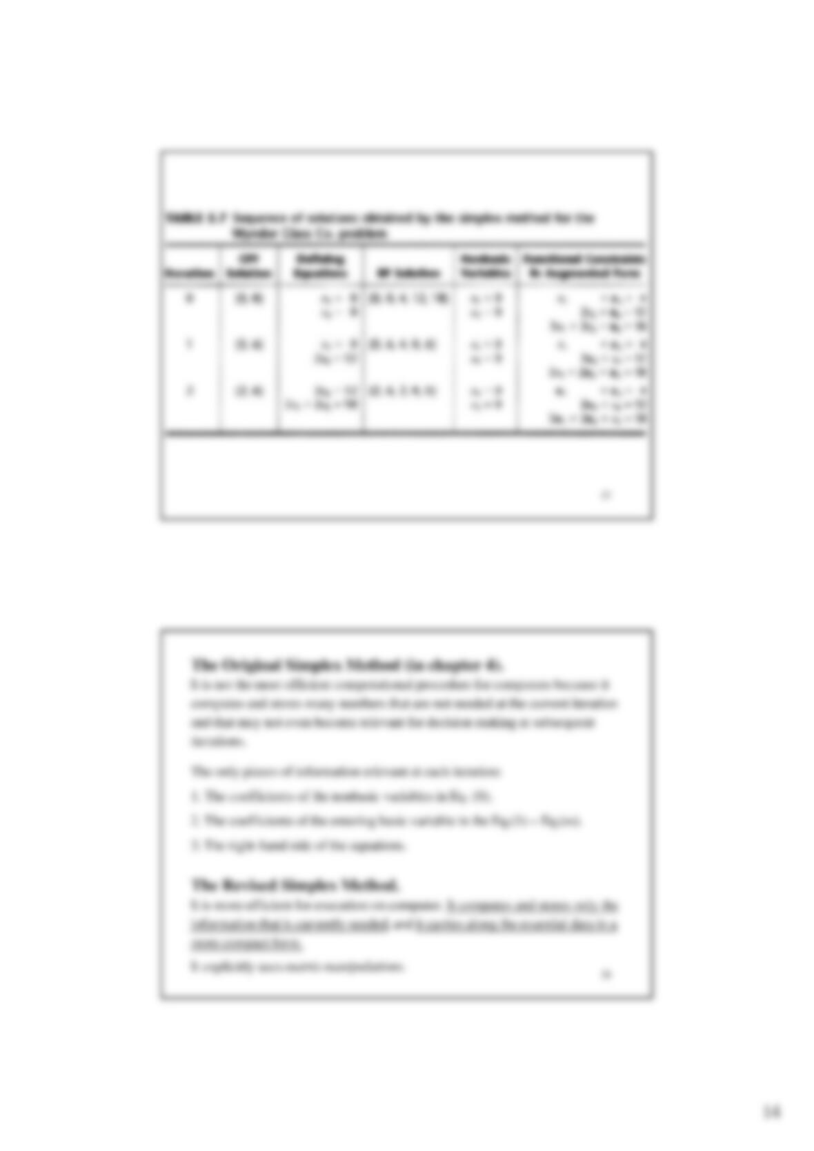
3. Matrix form solution procedure & avoid unnecessary computation
It streamlines the procedure considerably for computer
implementation. →Revised Simplex Method
Geometric ConceptGeometric Concept
(Geometrical Interpretation)(Geometrical Interpretation)
2 2 ––dimensionaldimensional
Algebraic ProcedureAlgebraic Procedure
(Algebraic Interpretation)(Algebraic Interpretation)
n n ––dimensionaldimensional
How the corner feasible solutions is identified algebraically?
The simplex method only searches on the corner feasible solutions.
2
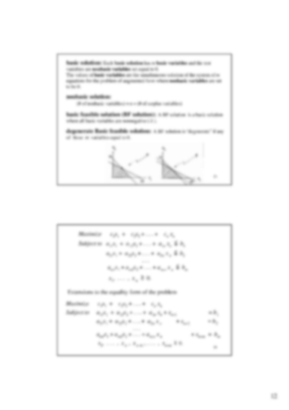
Maximize c1x1+c2x2+ . . . + cnxn
Subject to a11x1+a12x2+ . . . + a1nxn≦b1
a21x1+ a22x2+ . . . + a2n xn≦b2
. . .
am1x1+ am2x2+ . . . + am n xn≦bm
x1, . . . , xn≧0.
Extensions to the equality form of the problem
Maximize c1x1+c2x2+ . . . + cnxn
Subject to a11x1+a12x2+ . . . + a1nxn+ xn+1 = b1
a21x1+ a22x2+ . . . + a2n xn+ xn+2 = b2
. . .
am1x1+ am2x2+ . . . + am n xn+ xn+m= bm
x1, . . . , xn, xn +1 , . . . , xn+m≧0.
2
3
constraint boundary equation: (代數意義)
change inequalities ≤, ≥, = by = .
boundary of the feasible region: (幾何意義)
ai1x1+ ai2x2+ . . . + ainxn≦bi
⇒
ai1x1+ ai2x2+ . . . + ainxn= bi
xj≧0xj=0
⇒
constraint boundary equation
constraint boundary: (幾何意義)
It separates the points satisfying the constraint
from the points violating the constraint.
boundary: (幾何意義)
The boundary of the feasible region contains
just those feasible solutions that satisfy one or
more of the constraint boundary equations.
4
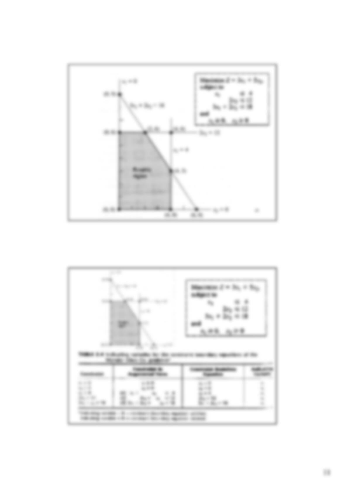
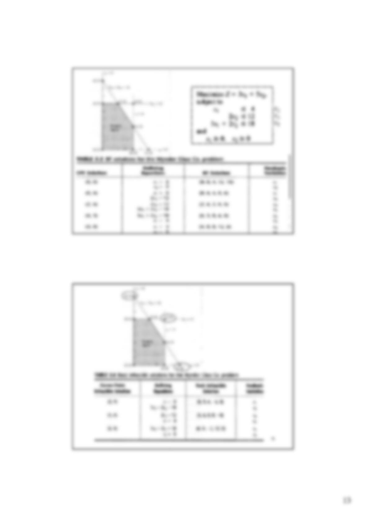
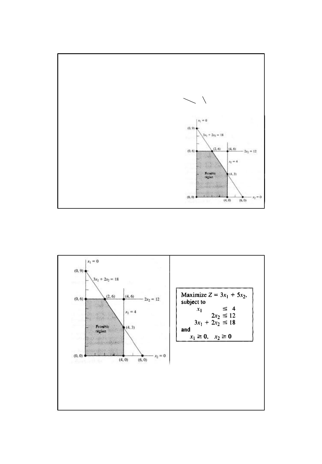
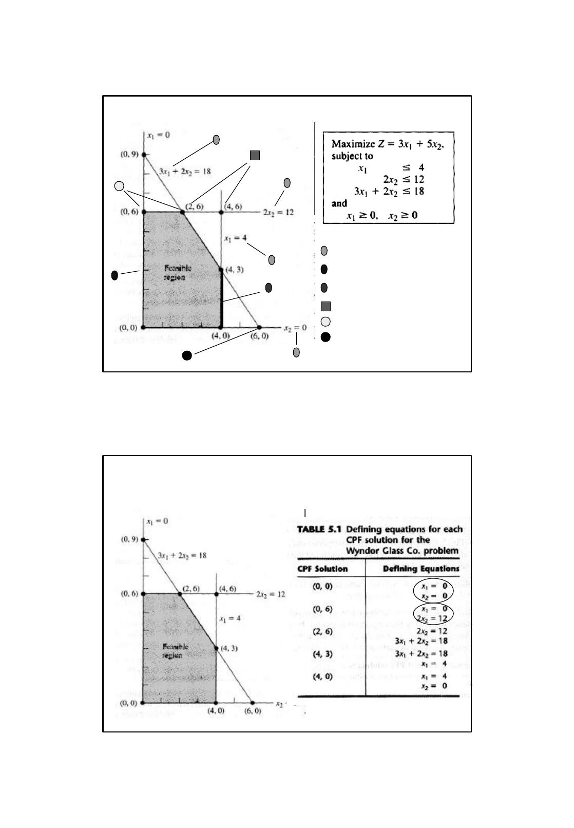
corner–point infeasible solution: (0, 9), (4, 6), (6, 0)
Wyndor Glass Co. problem
corner–point feasible solution: (0, 0), (0, 6), (2, 6), (4, 3), (4, 0)
corner–point solution: 如(0, 0), (0, 6), (0, 9), (2, 6), (4, 6) 等
3
5
constraint boundary equations
constraint boundary
corner–point solution
corner–point feasible solution
boundary of the feasible region
corner–point infeasible solution
6
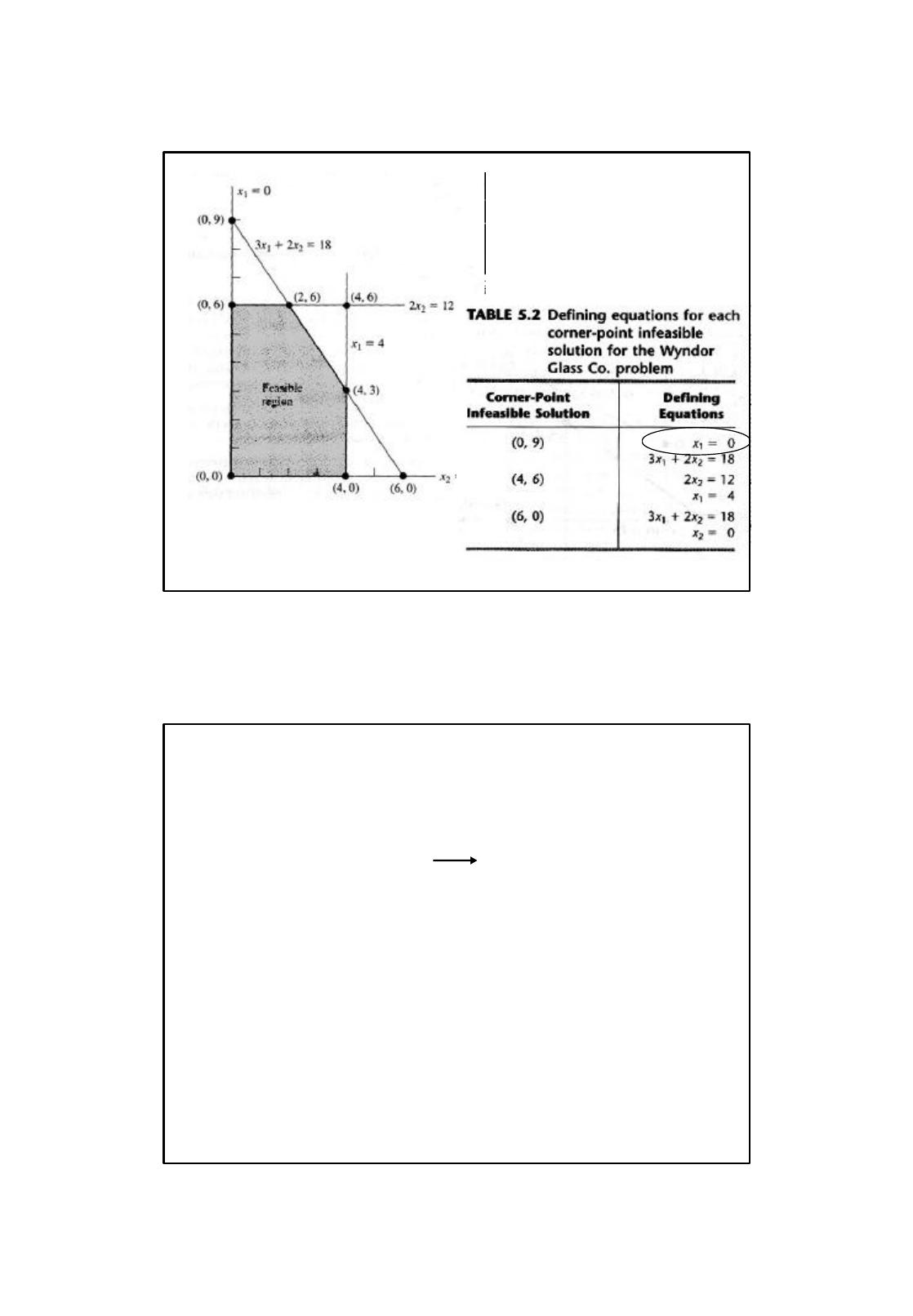
For any LP with ndecision variables, each CPF solutionis a
simultaneous solution of nconstraint boundary equations.
4
7
8
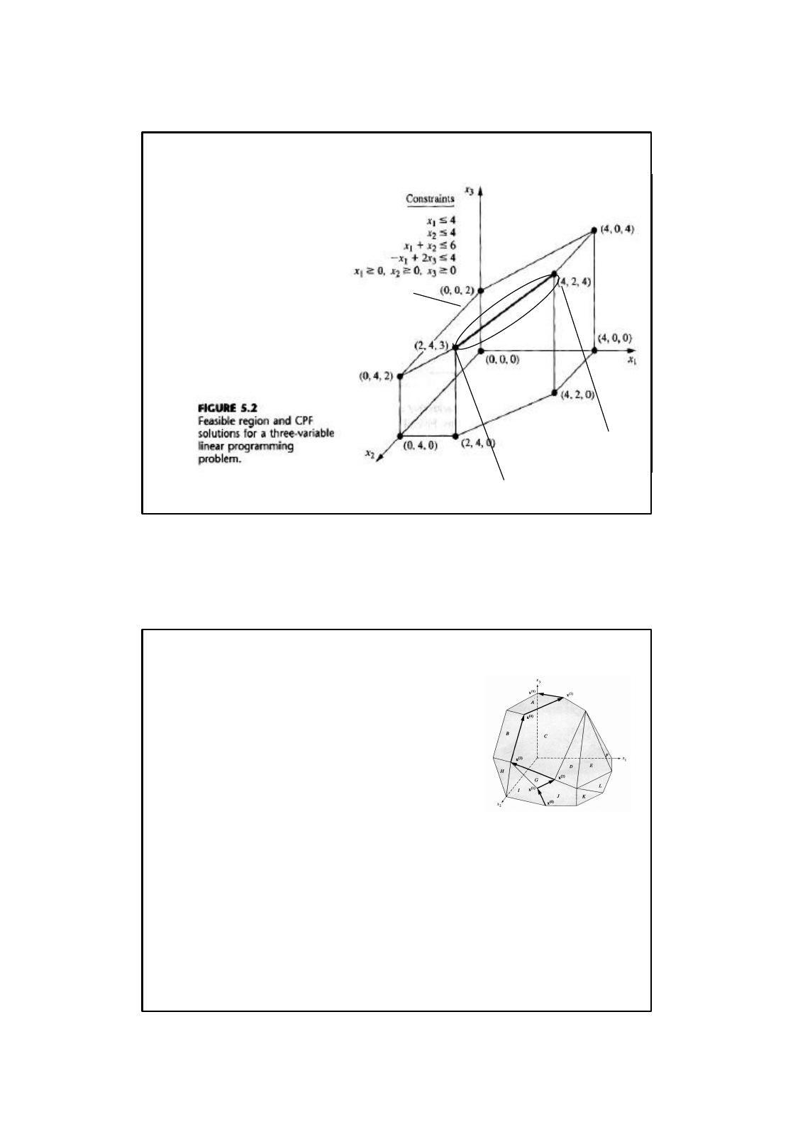
Two “adjacent”corner–point feasible solutions:
a. 幾何意義: 如(0, 0) 與(0, 6), (0, 0) 與(0, 4) (幾何意義)
b. 代數意義: Two “adjacent”corner–point feasible solutions 的defining
equations 只差一個不一樣
edge of a feasible region:
It lies at the intersection of n–1 constraint equations.
Simplex Method:
Move from one corner–point feasible solution to an adjacent
corner–point feasible solution.
Geometric interpretationGeometric interpretation Algebraic ProcedureAlgebraic Procedure
5
9
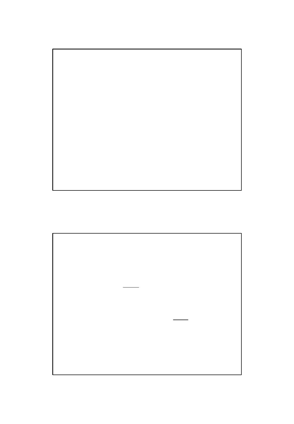
edge of a feasible region: It lies on
the line defined by x1+ x2= 6 and –x1+ 2x3= 4
Current CPF solution
The next CPF solution
(2, 4, 3): defining equations x2= 4, x1+ x2= 6, –x1+ 2x3= 4
Three ways lead to three adjacent CPF
solutions ↔three ways to remove a
Eq, from x2= 4, x1+ x2= 6,
–x1+ 2x3= 4
10
Consider a linear programming problem with bounded feasible region:
1. A CPF solution lies at the intersection of nconstraint boundaries (and
satisfies the other constraints as well.)
2. An edge of the feasible region is a feasible lines segment that lies at the
intersection of n–1 boundary boundaries, where each endpoint lies on one
additional constraint boundary (so that these endpoints are CPF solutions).
3. Two CPF solutions are adjacent if the line segment connecting them is an
edge of the feasible region. Emanating from each CPF solution are n such
edges, each one leading to one of the nadjacent CPF solutions.
4. Each iteration of the simplex method moves from the current CPF
solution to an adjacent one by moving along one of these edges.
Maximize c1x1+c2x2+ . . . + cnxn
Subject to a11x1+a12x2+ . . . + a1nxn≦b1
a21x1+ a22x2+ . . . + a2n xn≦b2
. . .
am1x1+ am2x2+ . . . + am n xn≦bm
x1, . . . , xn≧0.
6
11
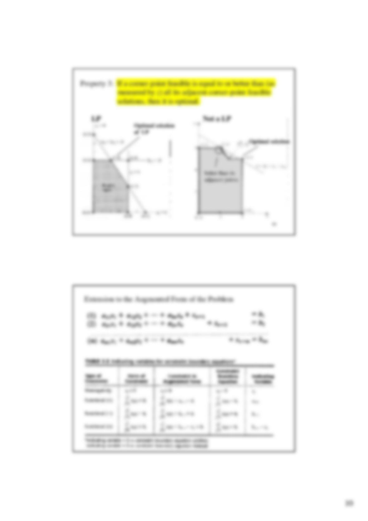
Property 1: (a) If there is exactly one optimal solution, then it must be a corner
point feasible solution.
Properties of CPF Solutions:
(b) If there are multiple optimal solutions, then at least
two must be adjacent corner–point feasible solution.
Proof: We will use a proof by contradiction. Suppose that x* is the unique
optimal solution and it is not a CPF solution.
x* is not a CPF solution.
⇒There exist two feasible solutions x’, x”such that x* lies on the
line segment [ x’, x”] where z1= cx’, z2= cx”.
⇒x* = αx’+ (1–α)x”, for α, 0 < α< 1.
⇒cx* = αcx’+ (1–α)cx”
⇒z* = αz1+ (1–α)z2
⇒One and only one of the following cases must hold.
z* = z1 = z2, z1< z* < z2, z2< z* < z1
⇒It contradicts to that x* is the unique optimal solution. Q.E.D.
12
Property 2: There are only a finite number of corner–point feasible
solution.
There are at most corner points.
!!
)!(
nm
nm
n
nm+
=
+
For example, m= 50, n= 50, .10
!50!50
!100
50
5050 29
≈=
+
mconstraints, ndecision variables →m + nconstraint boundary equations
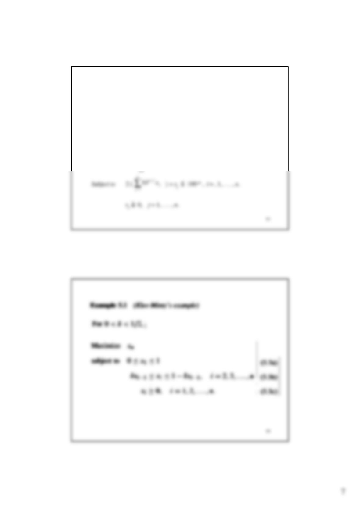
Example: How fast is the simplex method?
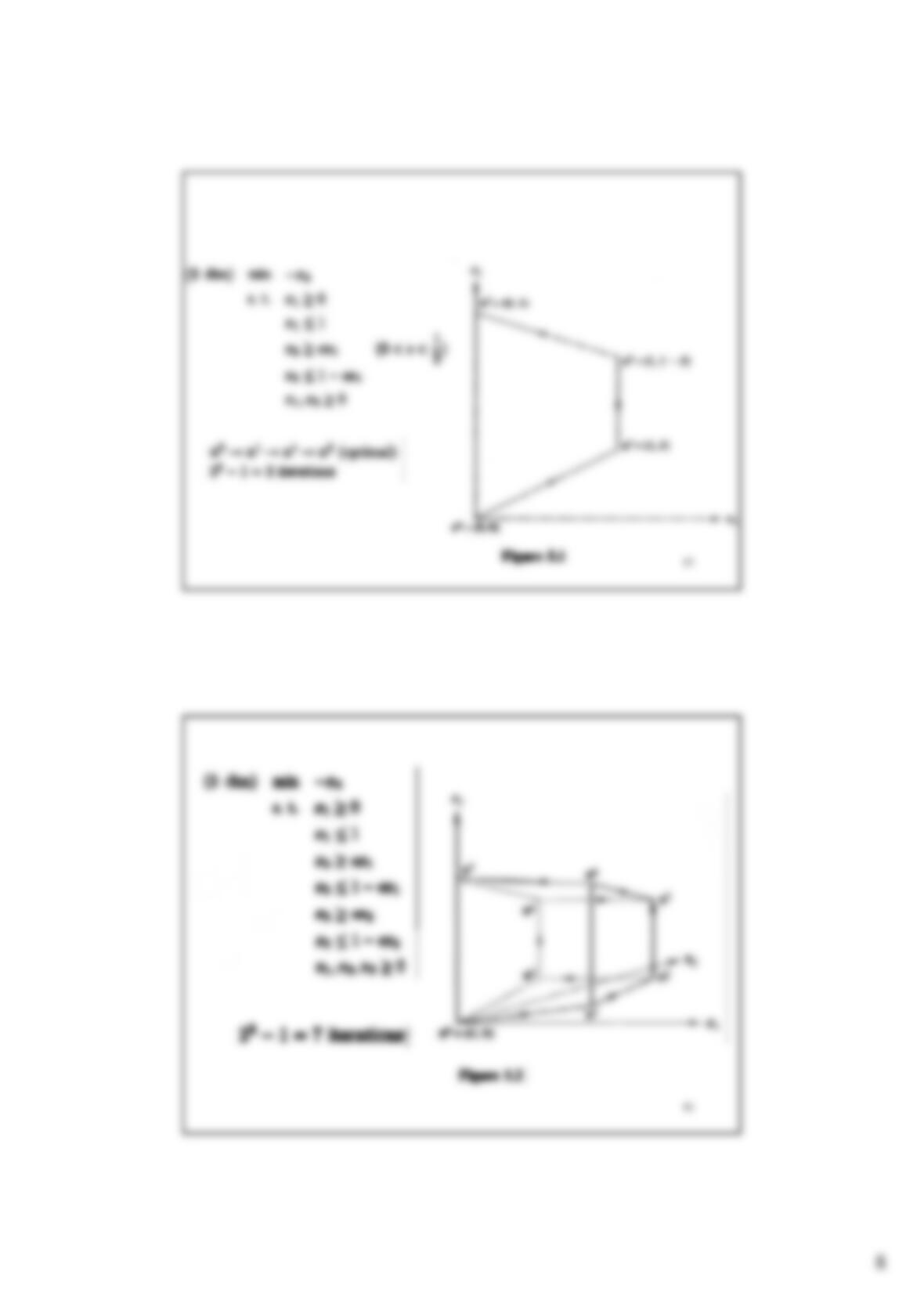
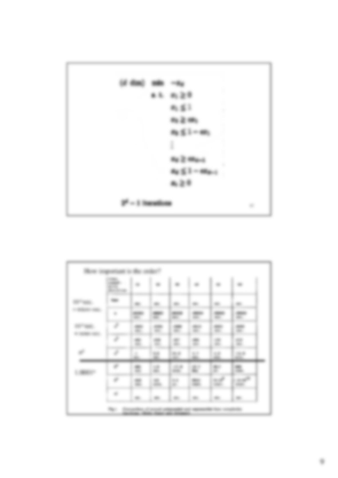
V. Klee and G.J. Minty (1972) have shown that in the process of solving the
following problem, the simplex method goes through 2n–1iterations. (For
example, at the rate of 100 iterations per second, the following problem with n
= 50 would take more than 300, 000 years to solve!) In general, the simplex
method works very well and it takes about 0.715 m0.9522 n0.3109 vertices.
Maximize z= ∑
−
n
jnx
10