68
CHAPTER 4
Exploratory Factor Analysis and Principal Components Analysis
Exploratory factor analysis (EFA) and principal components analysis (PCA) both are methods that are
used to help investigators represent a large number of relationships among normally distributed or scale
variables in a simpler (more parsimonious) way. Both of these approaches determine which, of a fairly
large set of items, “hang together” as groups or are answered most similarly by the participants. EFA also
can help assess the level of construct (factorial) validity in a dataset regarding a measure purported to
measure certain constructs. A related approach, confirmatory factor analysis, in which one tests very
specific models of how variables are related to underlying constructs (conceptual variables), requires
additional software and is beyond the scope of this book so it will not be discussed.
The primary difference, conceptually, between exploratory factor analysis and principal components
analysis is that in EFA one postulates that there is a smaller set of unobserved (latent) variables or
constructs underlying the variables actually observed or measured (this is commonly done to assess
validity), whereas in PCA one is simply trying to mathematically derive a relatively small number of
variables to use to convey as much of the information in the observed/measured variables as possible. In
other words, EFA is directed at understanding the relations among variables by understanding the
constructs that underlie them, whereas PCA is simply directed toward enabling one to derive fewer
variables to provide the same information that one would obtain from the larger set of variables.
There are actually a number of different ways of computing factors for factor analysis; in this chapter, we
will use only one of these methods, principal axis factor analysis (PA). We selected this approach
because it is highly similar mathematically to PCA. The primary difference, computationally, between
PCA and PA is that in the former the analysis typically is performed on an ordinary correlation matrix,
complete with the correlations of each item or variable with itself. In contrast, in PA factor analysis, the
correlation matrix is modified such that the correlations of each item with itself are replaced with a
“communality”—a measure of that item’s relation to all other items (usually a squared multiple
correlation). Thus, with PCA the researcher is trying to reproduce all information (variance and
covariance) associated with the set of variables, whereas PA factor analysis is directed at understanding
only the covariation among variables.
Conditions for Exploratory Factor Analysis and Principal Components Analysis
There are two main conditions necessary for factor analysis and principal components analysis. The first
is that there need to be relationships among the variables. Further, the larger the sample size, especially in
relation to the number of variables, the more reliable the resulting factors. Sample size is less crucial for
factor analysis to the extent that the communalities of items with the other items are high, or at least
relatively high and variable. Ordinary principal axis factor analysis should never be done if the number of
items/variables is greater than the number of participants.
Assumptions for Exploratory Factor Analysis and Principal Components Analysis
The methods of extracting factors and components that are used in this book do not make strong
distributional assumptions; normality is important only to the extent that skewness or outliers affect the
observed correlations or if significance tests are performed (which is rare for EFA and PCA). The
normality of the distribution can be checked by computing the skewness value of each variable.
Maximum likelihood estimation, which we will not cover, does require multivariate normality; the
variables need to be normally distributed and the joint distribution of all the variables should be normal.
Because both principal axis factor analysis and principal components analysis are based on correlations,
independent sampling is required and the variables should be related to each other (in pairs) in a linear
EXPLORATORY FACTOR ANALYSIS AND PRINCIPAL COMPONENTS ANALYSIS 69
fashion. The assumption of linearity can be assessed with matrix scatterplots, as shown in Chapter 2.
Finally, each of the variables should be correlated at a moderate level with some of the other variables.
Factor analysis and principal components analysis seek to explain or reproduce the correlation matrix,
which would not be a sensible thing to do if the correlations all hover around zero. Bartlett’s test of
sphericity addresses this assumption. However, if correlations are too high, this may cause problems with
obtaining a mathematical solution to the factor analysis.
• Retrieve your data file: hsbdataNew.sav.
Problem 4.1: Factor Analysis on Math Attitude Variables
In Problem 4.1, we perform a principal axis factor analysis on the math attitude variables. Factor analysis
is more appropriate than PCA when one has the belief that there are latent variables underlying the
variables or items measured. In this example, we have beliefs about the constructs underlying the math
attitude questions; we believe that there are three constructs: motivation, competence, and pleasure. Now,
we want to see if the items that were written to index each of these constructs actually do “hang together”;
that is, we wish to determine empirically whether participants’ responses to the motivation questions are
more similar to each other than to their responses to the competence items, and so on. Conducting factor
analysis can assist us in validating the data: if the data do fit into the three constructs that we believe exist,
then this gives us support for the construct validity of the math attitude measure in this sample. The
analysis is considered exploratory factor analysis even though we have some ideas about the structure of
the data because our hypotheses regarding the model are not very specific; we do not have specific
predictions about the size of the relation of each observed variable to each latent variable, etc. Moreover,
we “allow” the factor analysis to find factors that best fit the data, even if this deviates from our original
predictions.
4.1 Are there three constructs (motivation, competence, and pleasure) underlying the math attitude
questions?
To answer this question, we will conduct a factor analysis using the principal axis factoring method and
specify the number of factors to be three (because our conceptualization is that there are three math
attitude scales or factors: motivation, competence, and pleasure).
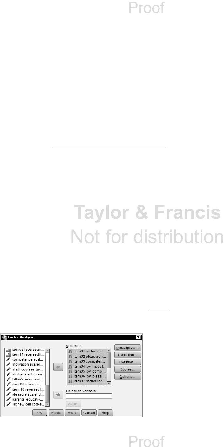
• Analyze → Dimension Reduction → Factor… to get Fig. 4.1.
• Next, select the variables item01 through item14. Do not include item04r or any of the other reversed
items because we are including the unreversed versions of those same items.
Fig. 4.1. Factor analysis.
70 CHAPTER 4
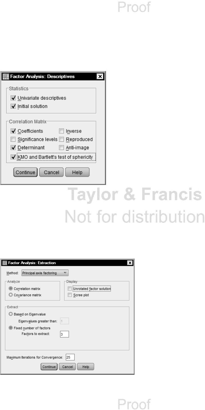
• Now click on Descriptives… to produce Fig. 4.2.
• Then click on the following: Initial solution and Univariate Descriptives (under Statistics),
Coefficients, Determinant, and KMO and Bartlett’s test of sphericity (under Correlation
Matrix).
• Click on Continue to return to Fig. 4.1.
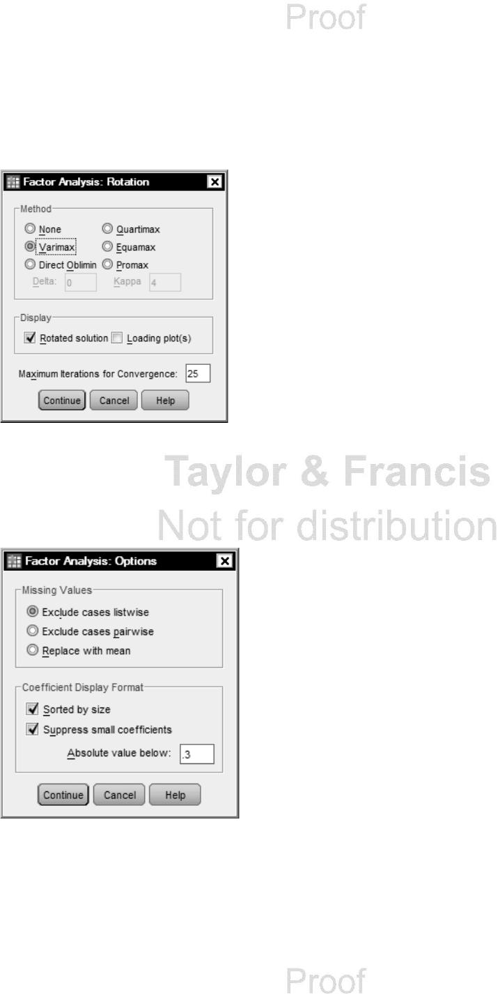
• Next, click on Extraction… This will give you Fig. 4.3.
• Select Principal axis factoring from the Method pull-down menu.
• Unclick Unrotated factor solution (under Display). We will examine this only in Problem 4.2. We
also usually would check the Scree plot box. However, again, we will request and interpret the scree
plot only in Problem 4.2.
• Click on Fixed number of factors under Extract, and type 3 in the box. This setting instructs the
computer to extract three math attitude factors.
• Click on Continue to return to Fig. 4.1.
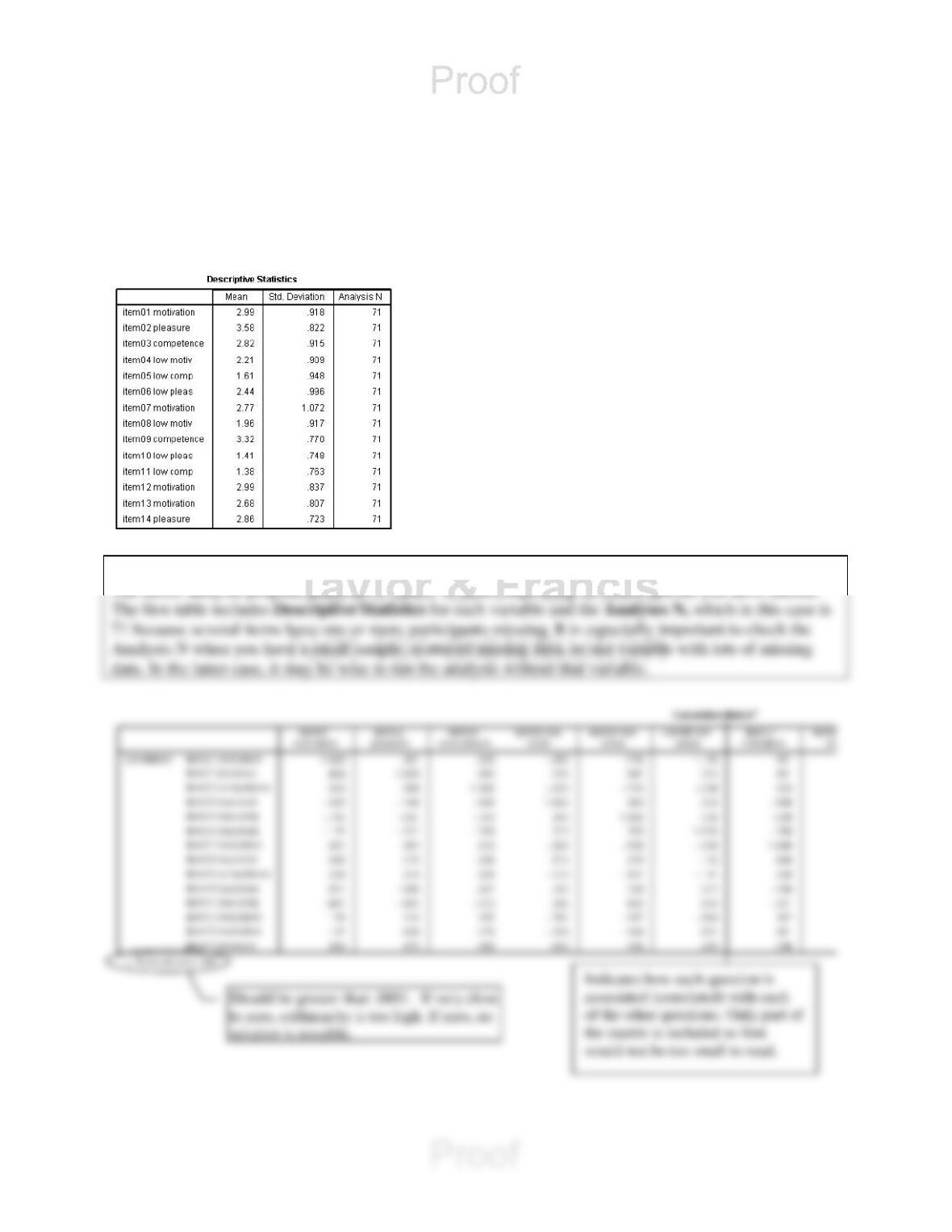
• Now click on Rotation… in Fig. 4.1, which will give you Fig. 4.4.
Fig. 4.2. Factor analysis: Descriptives.
Fig. 4.3. Extraction method to
produce principal axis factoring.
EXPLORATORY FACTOR ANALYSIS AND PRINCIPAL COMPONENTS ANALYSIS 71
• Click on Varimax, then make sure Rotated solution is also checked. Varimax rotation creates a
solution in which the factors are orthogonal (uncorrelated with one another), which can make results
easier to interpret and to replicate with future samples. If you believe that the factors (latent concepts)
are correlated, you could choose Direct Oblimin, which will provide an oblique solution allowing the
factors to be correlated.
• Click on Continue.
• Next, click on Options…, which will give you Fig. 4.5.
• Click on Sorted by size.
• Click on Suppress small coefficients and type .3 (point 3) in the Absolute Value below box (see
Fig. 4.5). Suppressing small factor loadings makes the output easier to read.
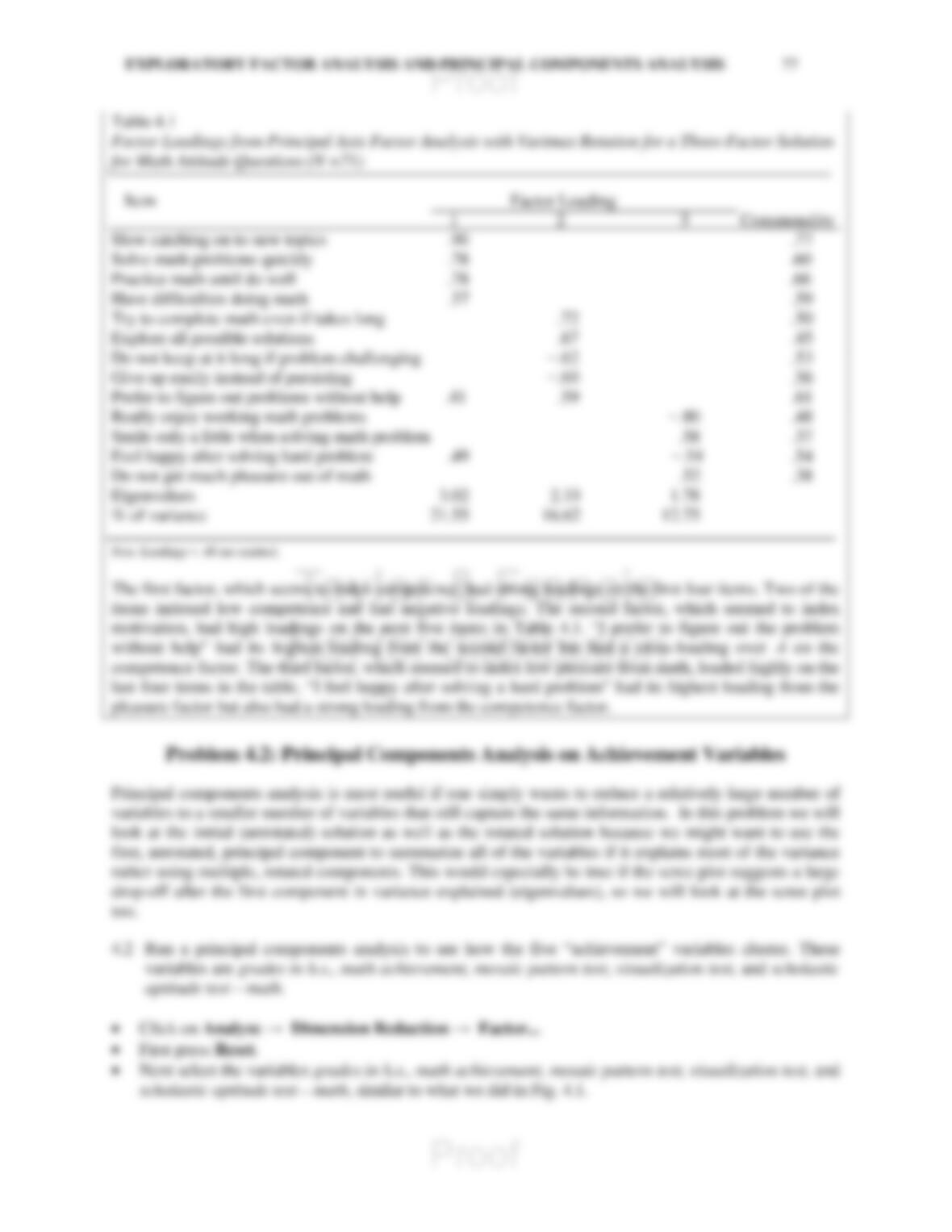
• Click on Continue then OK. Compare Output 4.1 with your output and syntax.
Output 4.1: Factor Analysis for Math Attitude Questions
FACTOR
/VARIABLES item01 item02 item03 item04 item05 item06 item07 item08 item09 item10 item11 item12
item13 item14
/MISSING LISTWISE
/ANALYSIS item01 item02 item03 item04 item05 item06 item07 item08 item09 item10 item11 item12
item13 item14
Fig. 4.4. Factor analysis: Rotation.
Fig. 4.5. Factor analysis: Options.
72 CHAPTER 4
/PRINT UNIVARIATE INITIAL CORRELATION DET KMO EXTRACTION ROTATION
/FORMAT SORT BLANK(.3)
/CRITERIA FACTORS(3) ITERATE(25)
/EXTRACTION PAF
/CRITERIA ITERATE(25)
/ROTATION VARIMAX
/METHOD=CORRELATION.
Factor Analysis
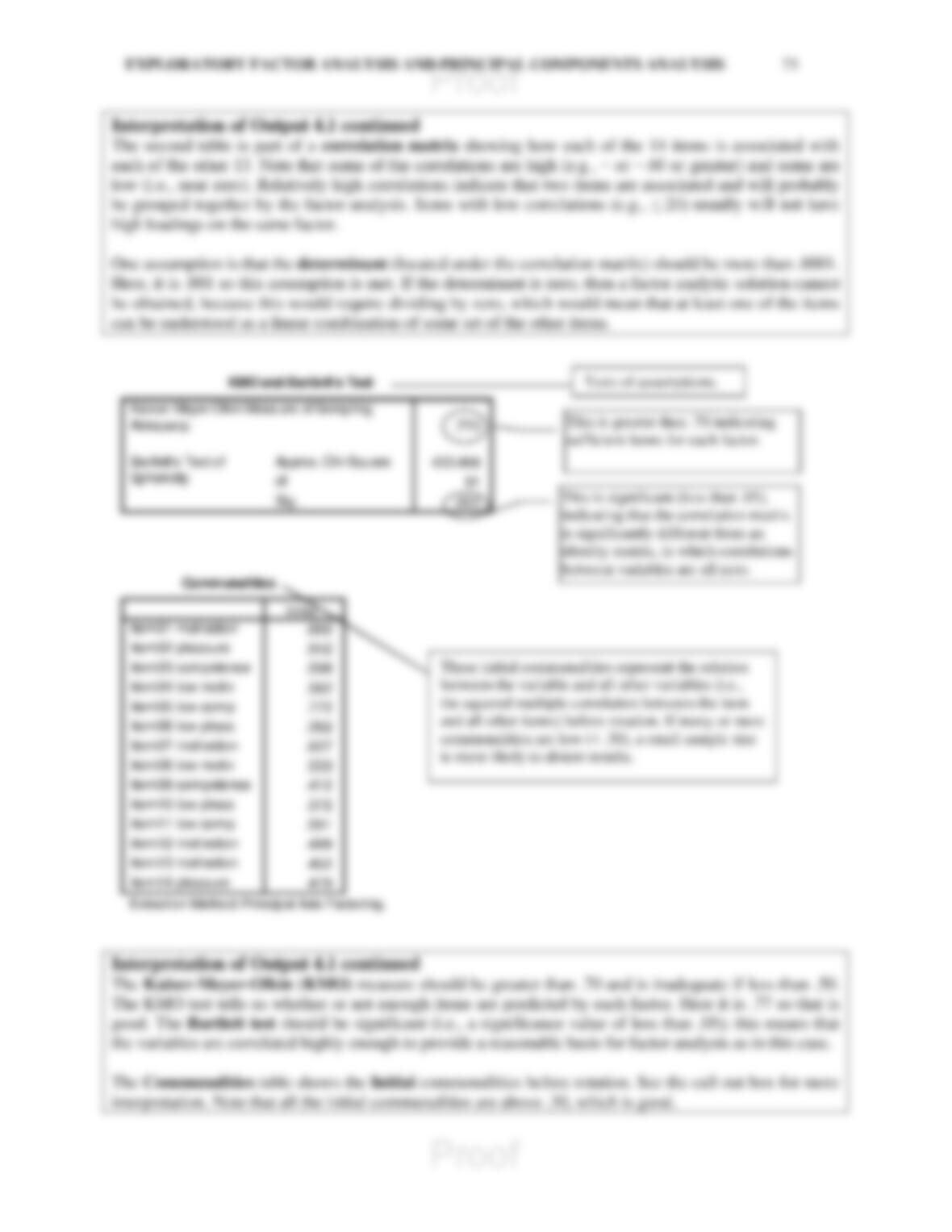
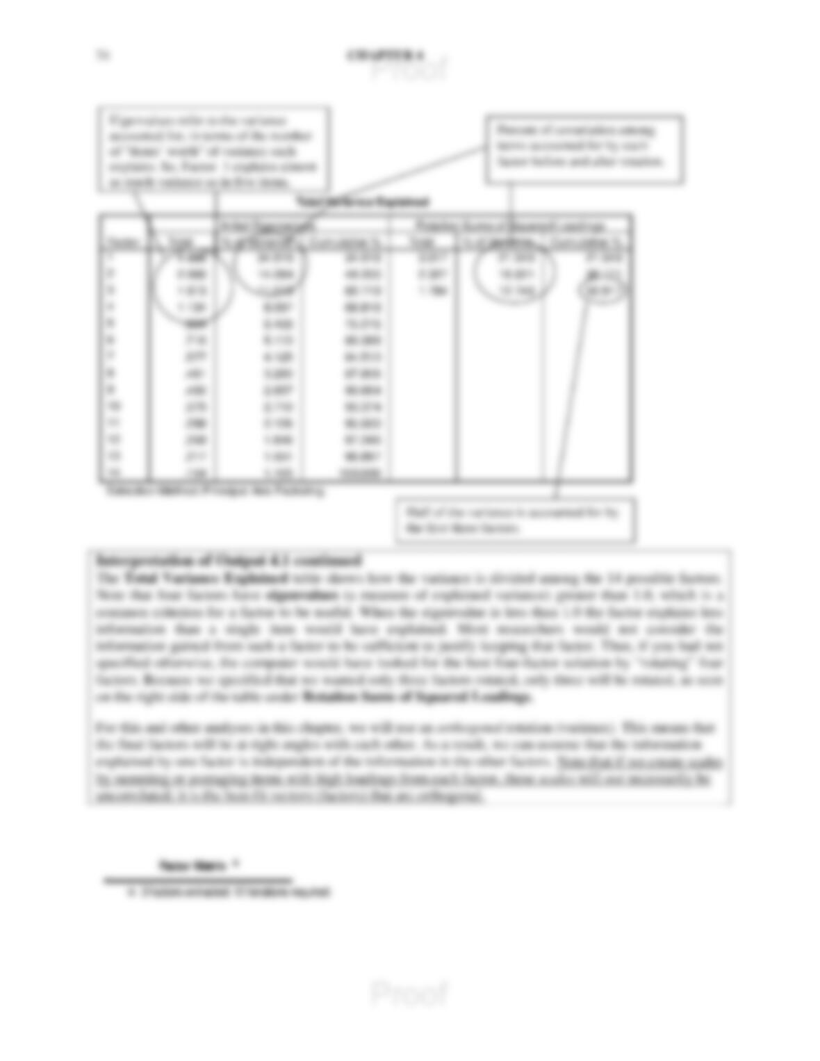
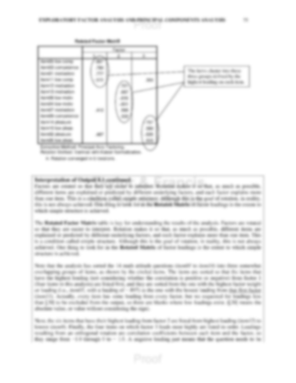
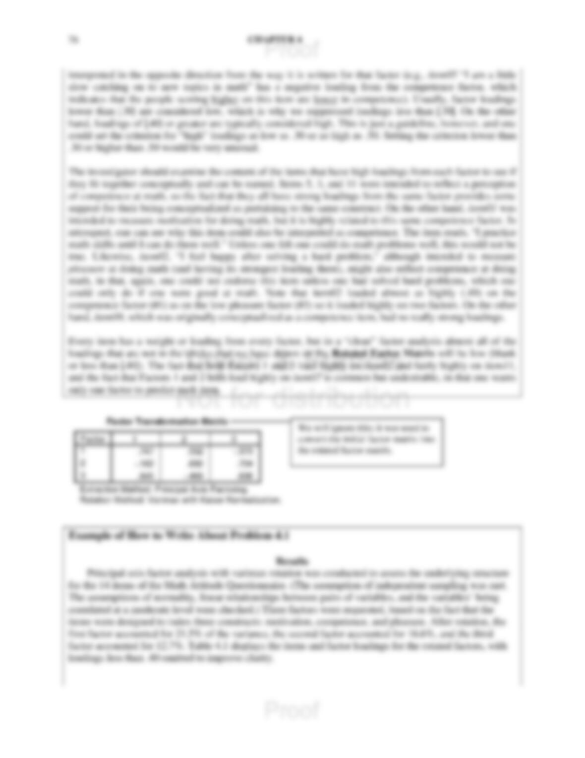
Interpretation of Output 4.1