Intermediate Macroeconomics
Lecture 4 – Growth models beyond Solow
Zs´ofia L. B´ar´any
Sciences Po
2014 February

Recap of Solow model
Ikey: the description of the dynamic evolution of saving –
investment – capital accumulation
Iprediction: each economy converges to its steady state which
features
Iconstant capital and output per worker
Iconstant consumption per worker
Ioutput and consumption only grow on the path to the steady
state, during the transition
Ichanges in the saving rate, the growth rate of population, and
the level of technology change the steady state
I→maybe sustained productivity growth leads to a sustained
growth in output per worker?

The Solow model with technological progress
Ithe basic Solow model with constant technology cannot
explain long-run growth in output per head
Ibut one of the key reasons why our living standard is much
higher than a century ago is technological progress
Iwe next extend the basic Solow model to allow for
technological progress
Itechnological progress: given the capital and labor inputs, an
improvement in technology leads to an increase in output
Iin general technological progress can be labor-augmenting,
capital-augmenting or neutral
Iwe will focus on the type of technological progress that is
labor-augmenting: it increases the efficiency, the productivity
of workers

Labor augmenting technological progress
Until now the production function was given by:
Y=zF (K,N)
here zis total factor productivity (TFP), increases in zincrease
the productivity of both labor and capital →neutral technological
progress
A labor-augmenting technology yields the following production
function:
Y=F(K,AN)
where Ais the technology →assume that it grows at constant rate
g:At+1 =At(1 + g)

An example: the Cobb-Douglas production function
we can write it as:
Y=zK αN1−α
this is equivalent to
Y=Kα(AN)1−α
if z=A1−α.
In the case of a Cobb-Douglas production function, neutral and
labor-augmenting technological progress are equivalent.
For other neoclassical production functions this is not the case.
A trick to simplifying our model
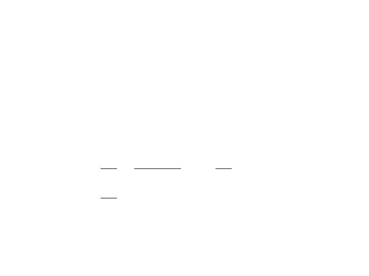
In the standard Solow model we converted every variable to its per
worker version:
Y=zF (K,N)⇒y=zf (k)
Here, in the model with labor-augmenting technological progress,
we convert everything into efficiency worker units:
˜y≡Y
AN =F(K,AN)
AN =FK
AN ,1=f(˜
k)
˜
k≡K
AN
we can do this (just as before) due to the constant returns to scale
property of F.

Finding the equilibrium of the model
1. Write down the capital accumulation equation
Kt+1 = (1 −d)Kt+It
2. Use the clearing of the capital market: It=St=sYt
Kt+1 = (1 −d)Kt+sF (Kt,AtNt)
3. Convert everything into efficiency units of labor
4. Analyze what happens to ˜
kover time
The capital accumulation equation
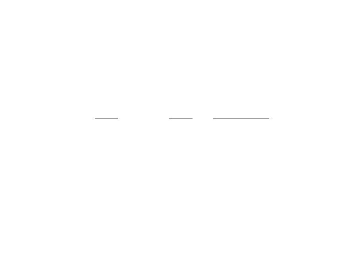
need to convert the following into efficiency labor units:
Kt+1 = (1 −d)Kt+sF (Kt,AtNt)
divide by AtNtand manipulate:
Kt+1
AtNt
= (1 −d)Kt
AtNt
+sF(Kt,AtNt)
AtNt
At+1Nt+1
At+1Nt+1
Kt+1
AtNt
= (1 −d)˜
kt+sf(˜
kt)
(1 + g)At(1 + n)Nt
AtNt
Kt+1
At+1Nt+1
= (1 −d)˜
kt+sf (˜
kt)
(1 + g)(1 + n)
| {z }
≈(1+g+n)
˜
kt+1 =(1 −d)˜
kt+sf (˜
kt)
The capital accumulation equation
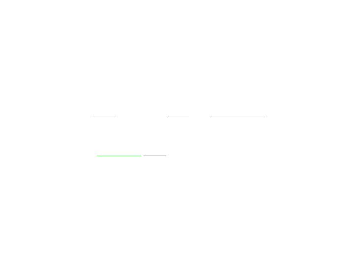
need to convert the following into efficiency labor units:
Kt+1 = (1 −d)Kt+sF (Kt,AtNt)
divide by AtNtand manipulate:
Kt+1
AtNt
= (1 −d)Kt
AtNt
+sF(Kt,AtNt)
AtNt
At+1Nt+1
At+1Nt+1
Kt+1
AtNt
= (1 −d)˜
kt+sf(˜
kt)
(1 + g)At(1 + n)Nt
AtNt
Kt+1
At+1Nt+1
= (1 −d)˜
kt+sf (˜
kt)
(1 + g)(1 + n)
| {z }
≈(1+g+n)
˜
kt+1 =(1 −d)˜
kt+sf (˜
kt)

The capital accumulation equation
need to convert the following into efficiency labor units:
Kt+1 = (1 −d)Kt+sF (Kt,AtNt)
divide by AtNtand manipulate:
Kt+1
AtNt
= (1 −d)Kt
AtNt
+sF(Kt,AtNt)
AtNt
At+1Nt+1
At+1Nt+1
Kt+1
AtNt
= (1 −d)˜
kt+sf(˜
kt)
(1 + g)At(1 + n)Nt
AtNt
Kt+1
At+1Nt+1
= (1 −d)˜
kt+sf (˜
kt)
(1 + g)(1 + n)
| {z }
≈(1+g+n)
˜
kt+1 =(1 −d)˜
kt+sf (˜
kt)
The capital accumulation equation
need to convert the following into efficiency labor units:
Kt+1 = (1 −d)Kt+sF (Kt,AtNt)
divide by AtNtand manipulate:
Kt+1
AtNt
= (1 −d)Kt
AtNt
+sF(Kt,AtNt)
AtNt
At+1Nt+1
At+1Nt+1
Kt+1
AtNt
= (1 −d)˜
kt+sf(˜
kt)
(1 + g)At(1 + n)Nt
AtNt
Kt+1
At+1Nt+1
= (1 −d)˜
kt+sf (˜
kt)
(1 + g)(1 + n)
| {z }
≈(1+g+n)
˜
kt+1 =(1 −d)˜
kt+sf (˜
kt)
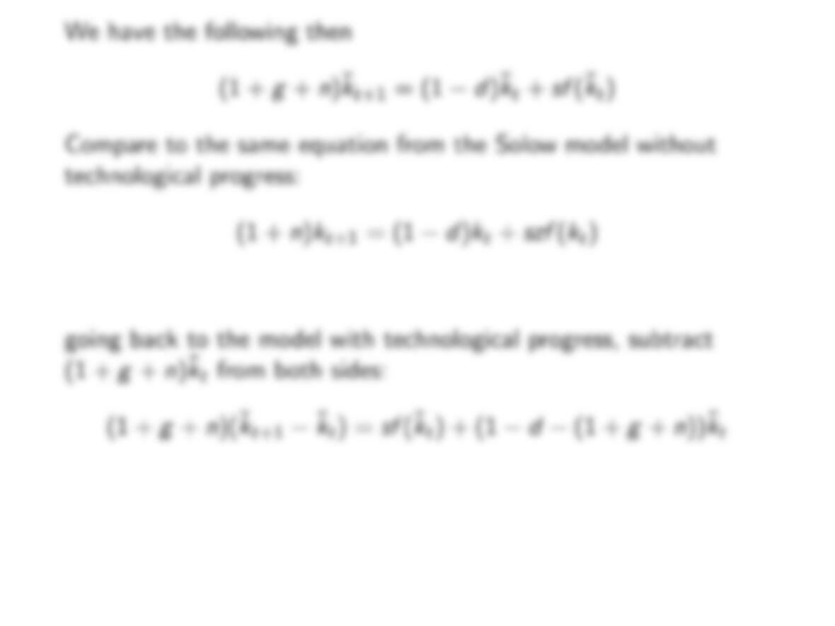
going back to the model with technological progress, subtract
(1 + g+n)˜
ktfrom both sides:
(1 + g+n)(˜
kt+1 −˜
kt) = sf (˜
kt) + (1 −d−(1 + g+n))˜
kt
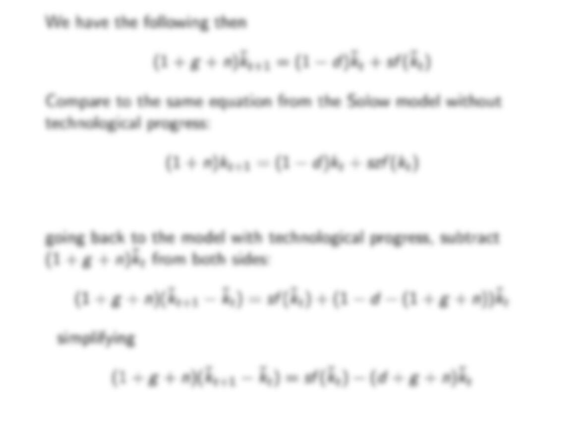
simplifying
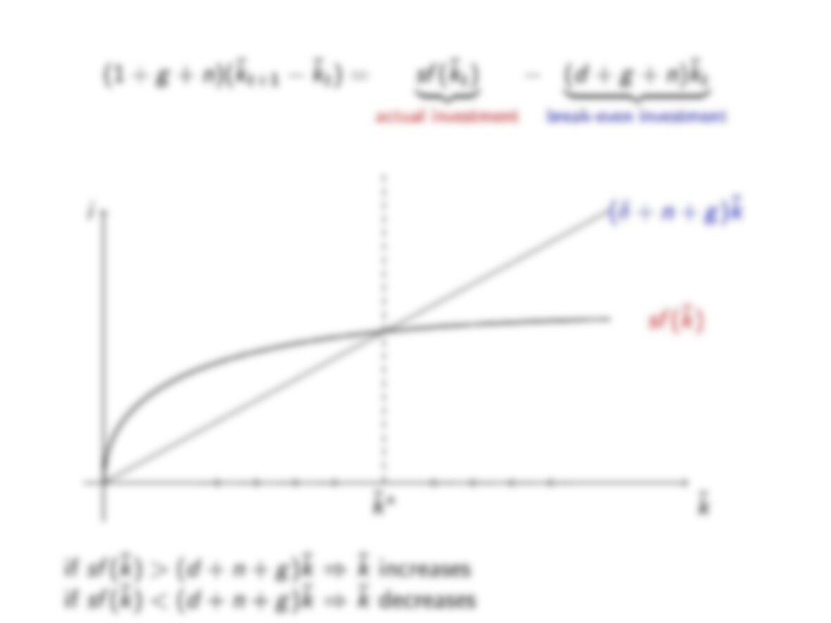
(1 + g+n)(˜
kt+1 −˜
kt) = sf (˜
kt)−(d+g+n)˜
kt
simplifying
(1 + g+n)(˜
kt+1 −˜
kt) = sf (˜
kt)−(d+g+n)˜
kt
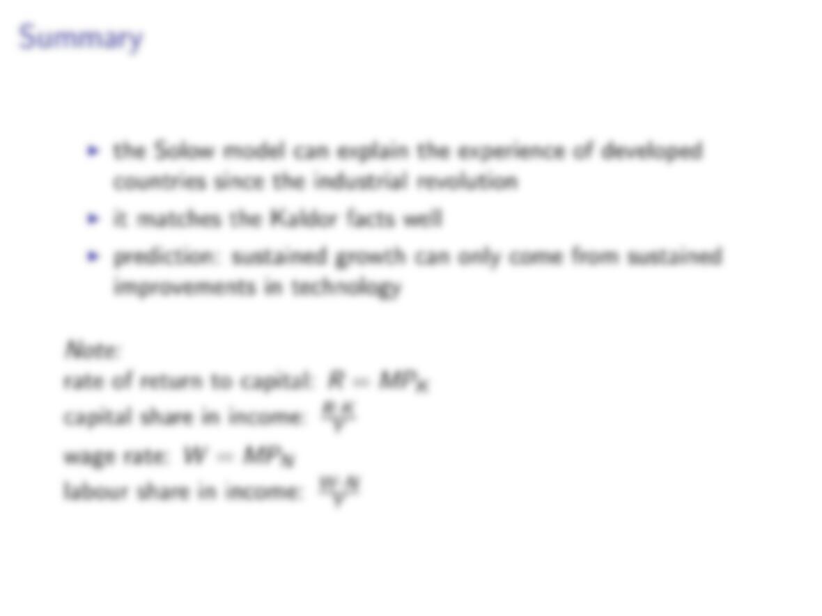
Do the predictions of the Solow model with technological progress
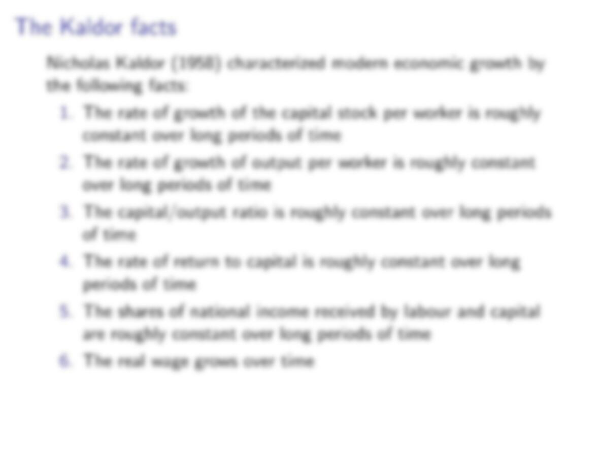
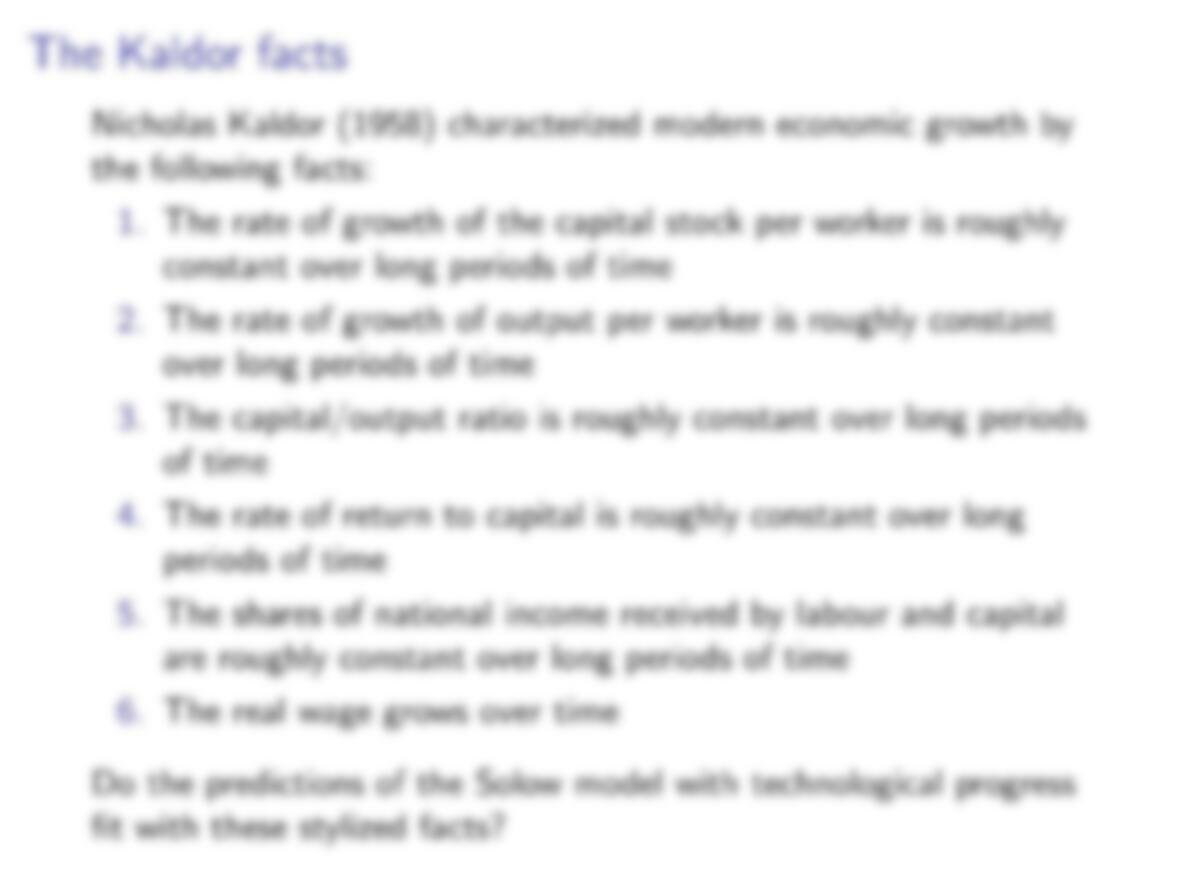
fit with these stylized facts?
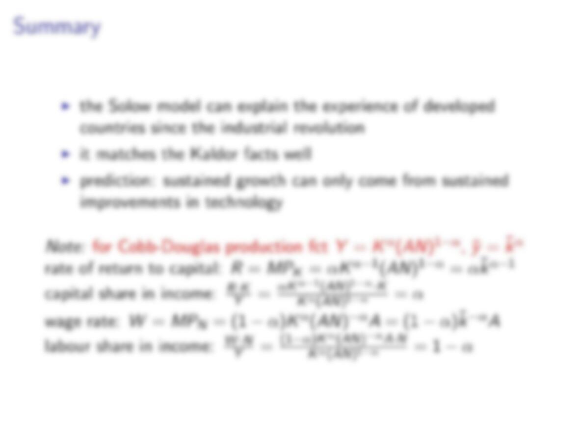
for Cobb-Douglas production fct Y=Kα(AN)1−α, ˜y=˜
kα
=αKα−1(AN)1−α=α˜
kα−1
=αKα−1(AN)1−α·K
Kα(AN)1−α=α
= (1 −α)Kα(AN)−αA= (1 −α)˜
k−αA
=(1−α)Kα(AN)−αA·N
Kα(AN)1−α= 1 −α

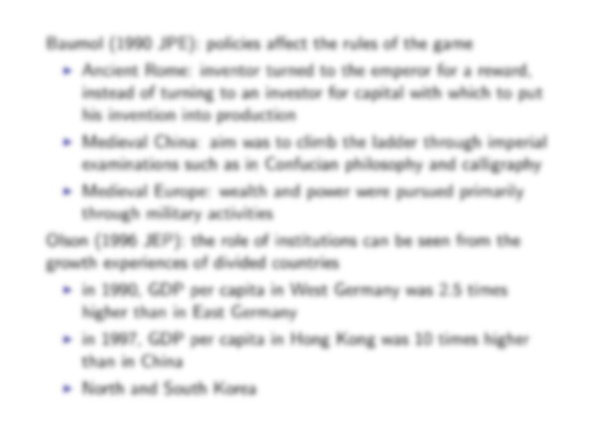
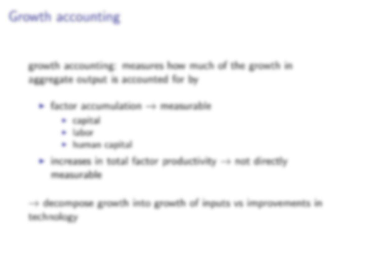
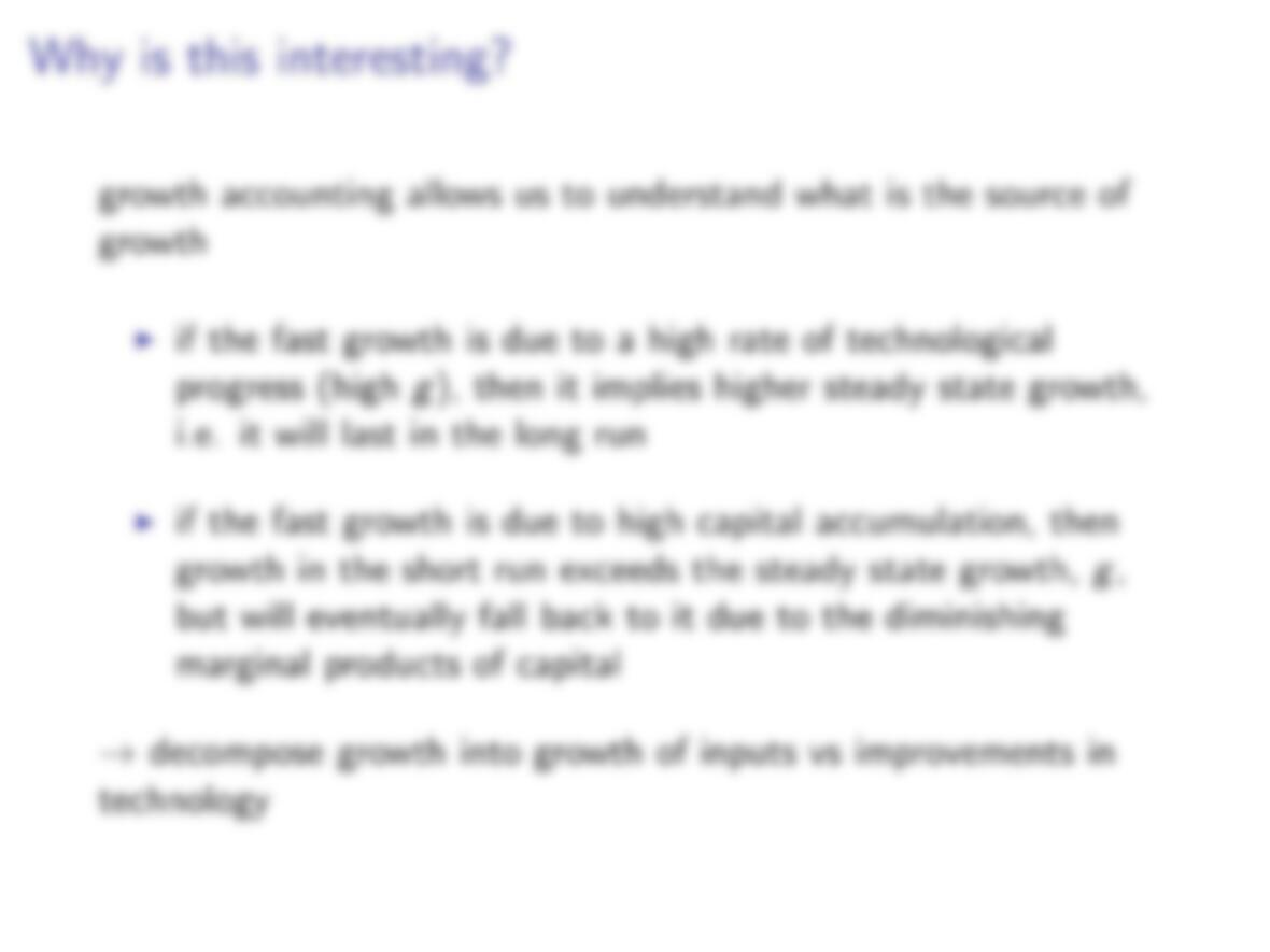
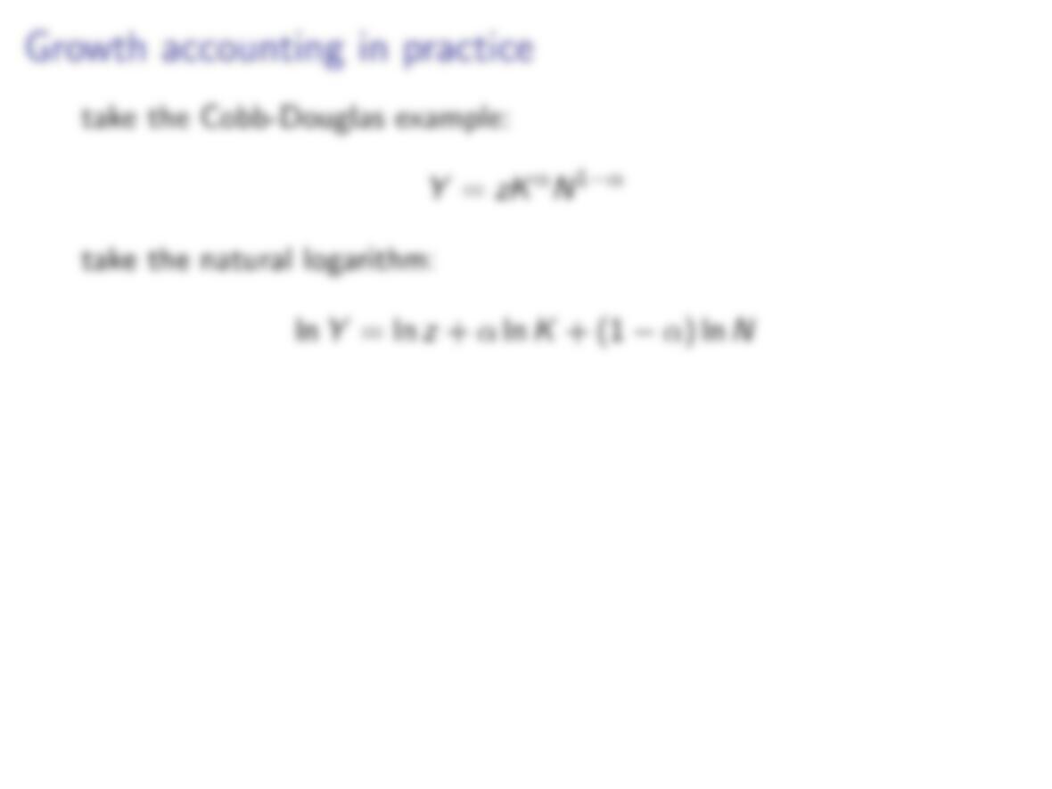
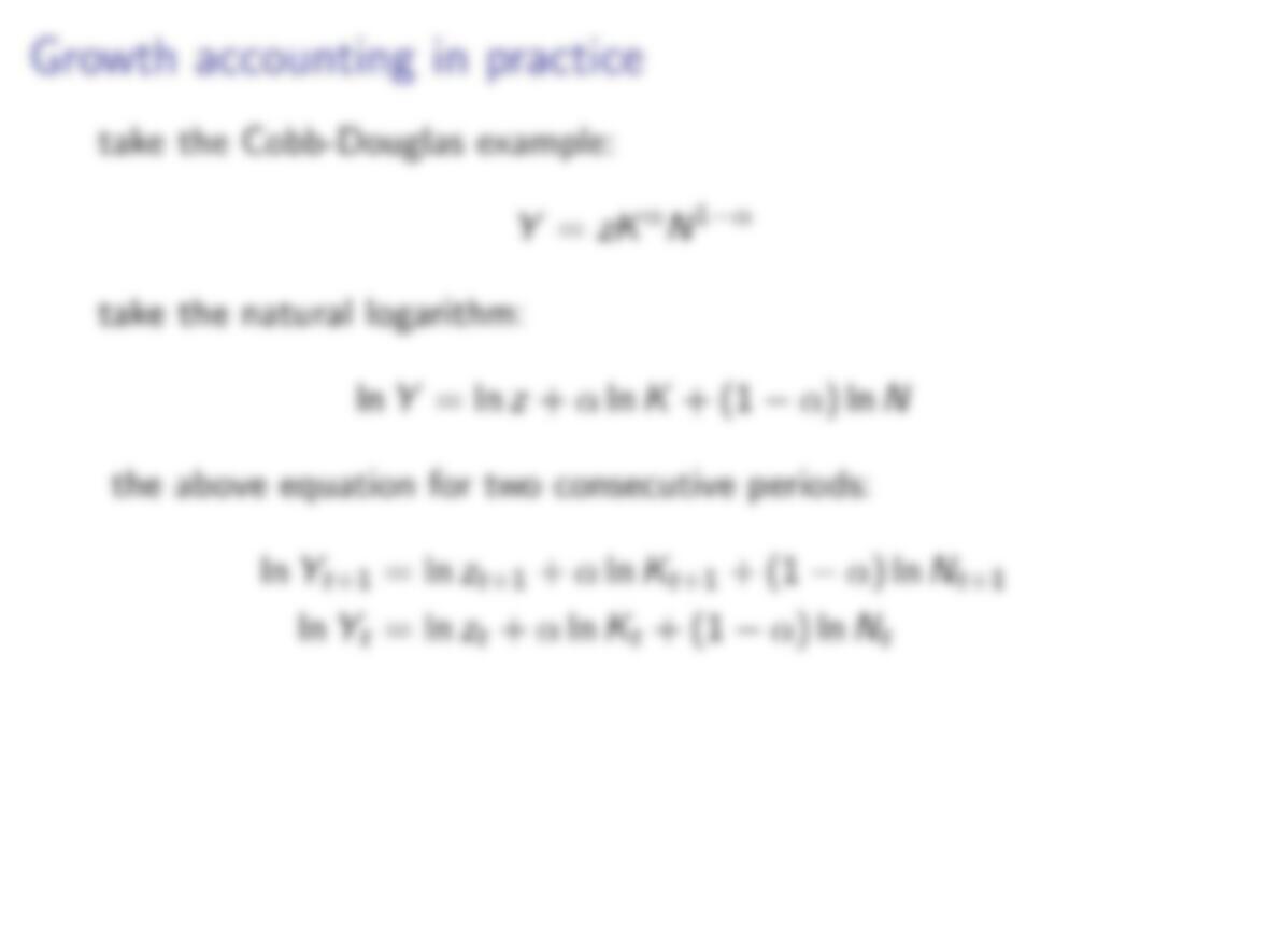
the above equation for two consecutive periods:
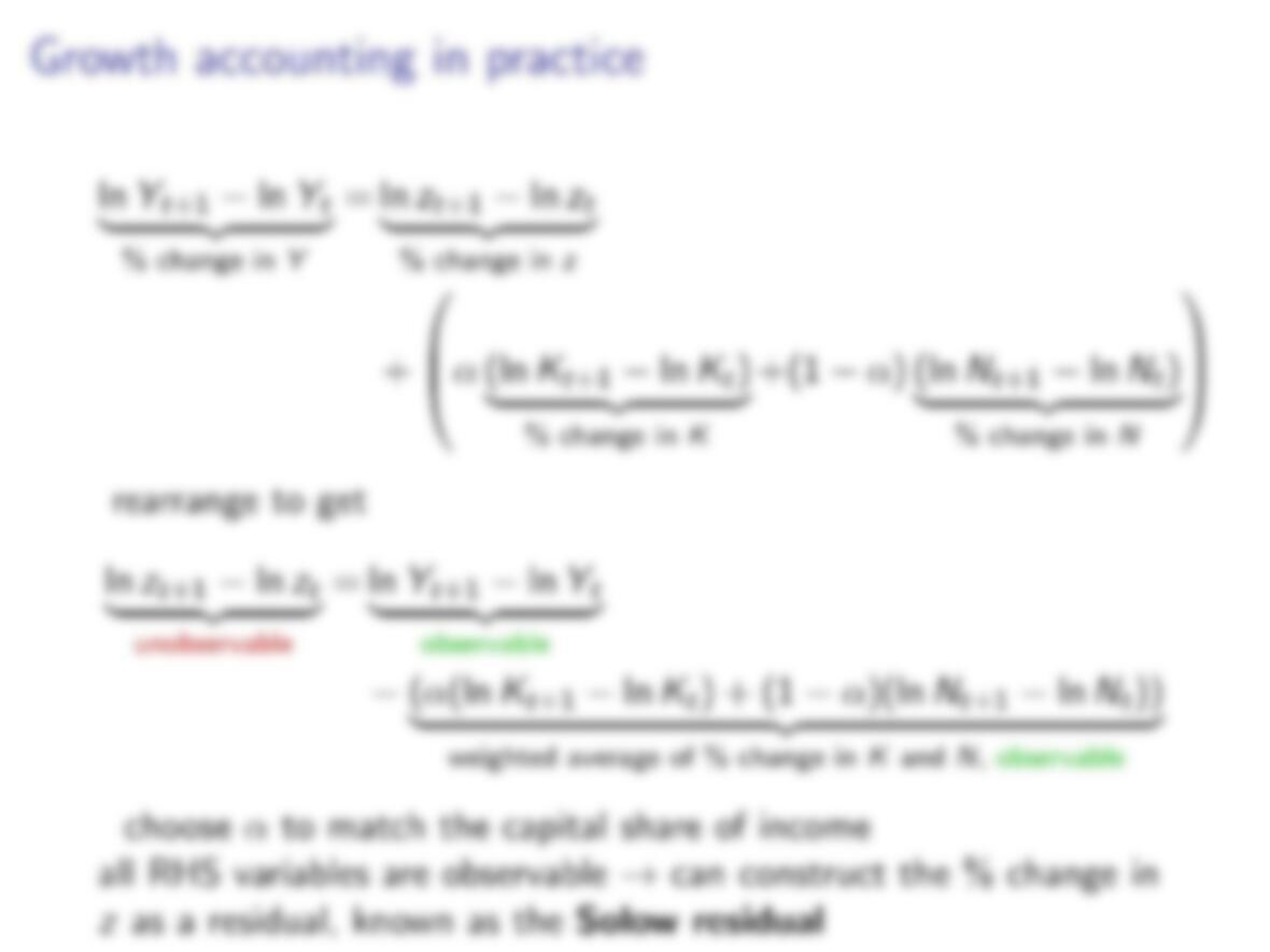
ln Yt+1 = ln zt+1 +αln Kt+1 + (1 −α) ln Nt+1
ln Yt= ln zt+αln Kt+ (1 −α) ln Nt
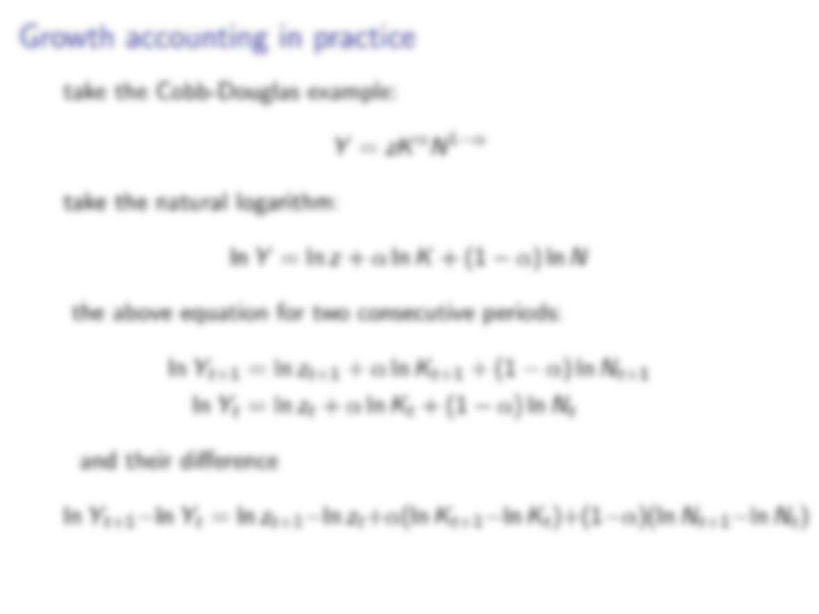
and their difference
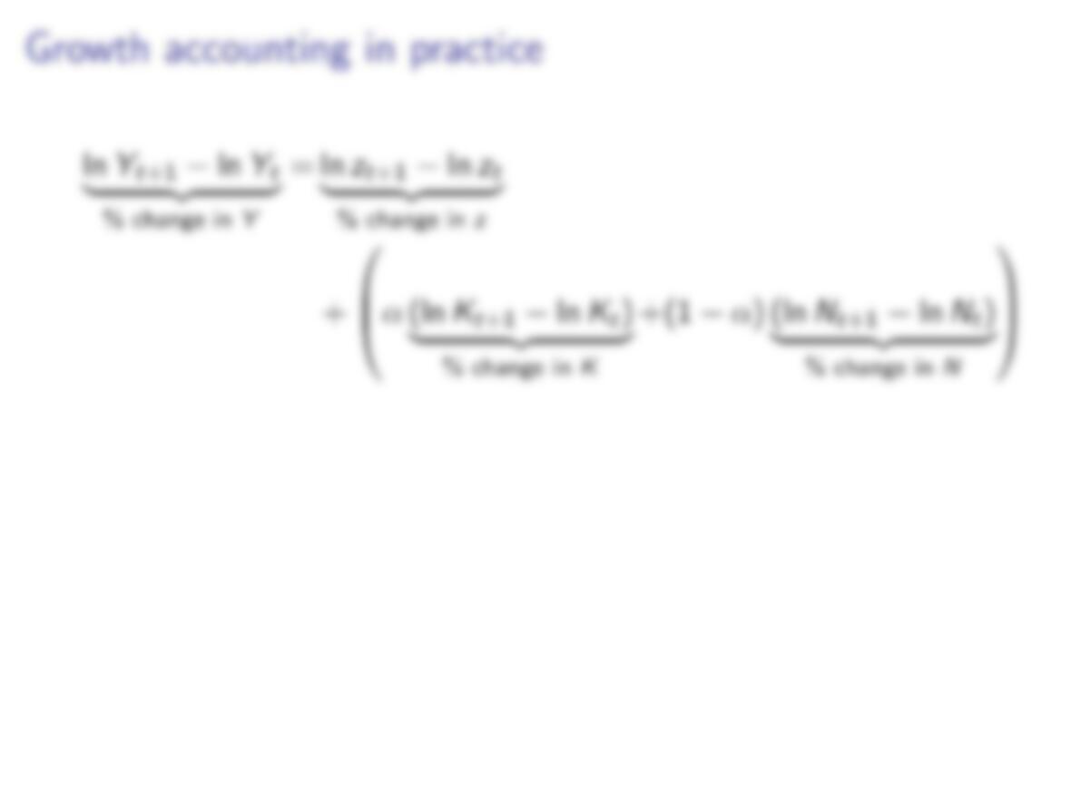
ln Yt+1−ln Yt= ln zt+1−ln zt+α(ln Kt+1−ln Kt)+(1−α)(ln Nt+1−ln Nt)
and their difference
ln Yt+1−ln Yt= ln zt+1−ln zt+α(ln Kt+1−ln Kt)+(1−α)(ln Nt+1−ln Nt)
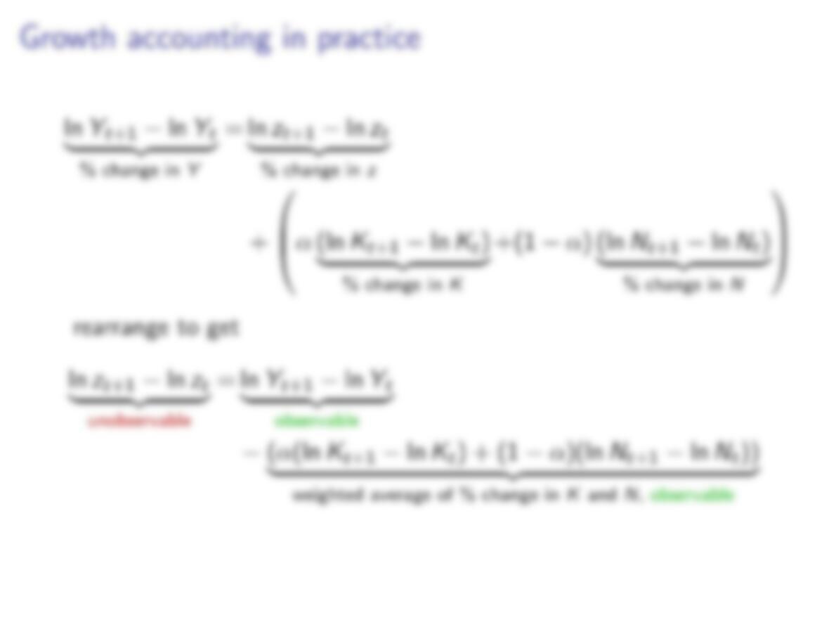
rearrange to get
ln zt+1 −ln zt
| {z }
unobservable
= ln Yt+1 −ln Yt
| {z }
observable
−(α(ln Kt+1 −ln Kt) + (1 −α)(ln Nt+1 −ln Nt))
| {z }
weighted average of % change in Kand N,observable
choose αto match the capital share of income
all RHS variables are observable →can construct the % change in
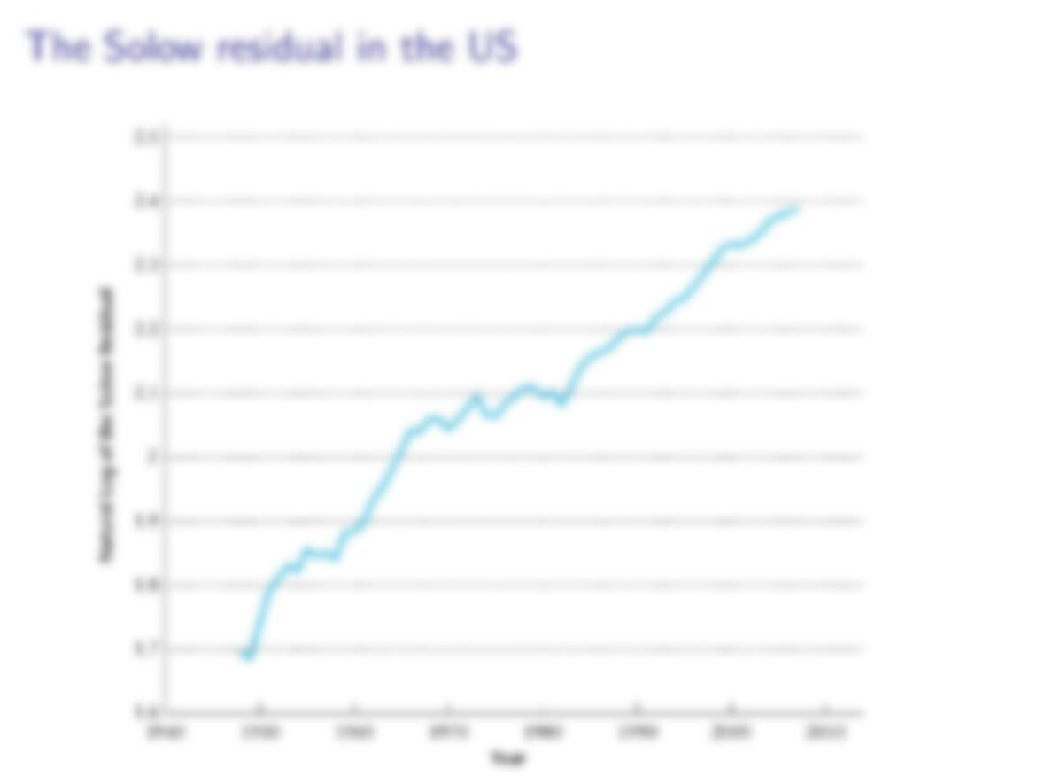
zas a residual, known as the Solow residual
choose αto match the capital share of income
all RHS variables are observable →can construct the % change in
zas a residual, known as the Solow residual
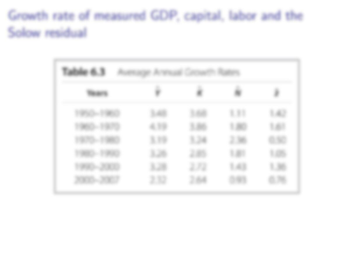
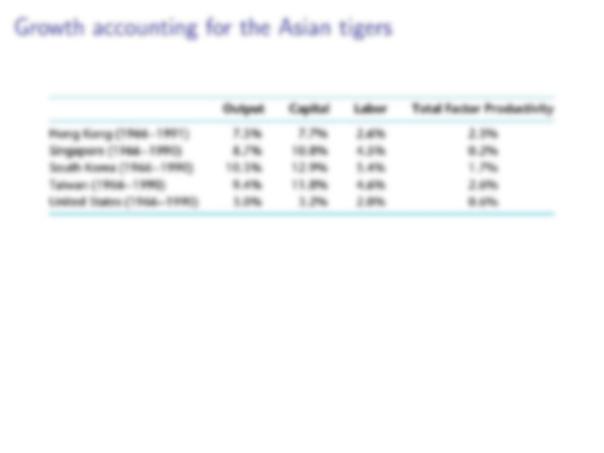
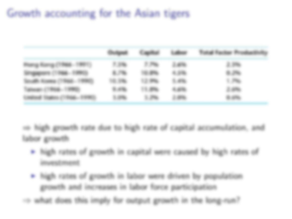
⇒high growth rate due to high rate of capital accumulation, and
labor growth
Ihigh rates of growth in capital were caused by high rates of
investment
Ihigh rates of growth in labor were driven by population
growth and increases in labor force participation
⇒what does this imply for output growth in the long-run?
z
z
z
z
zrich
zrich
zpoor
zpoor
zrich
zpoor 1
1−α
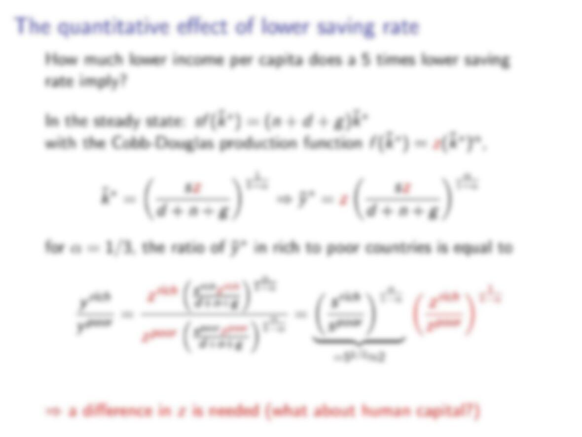
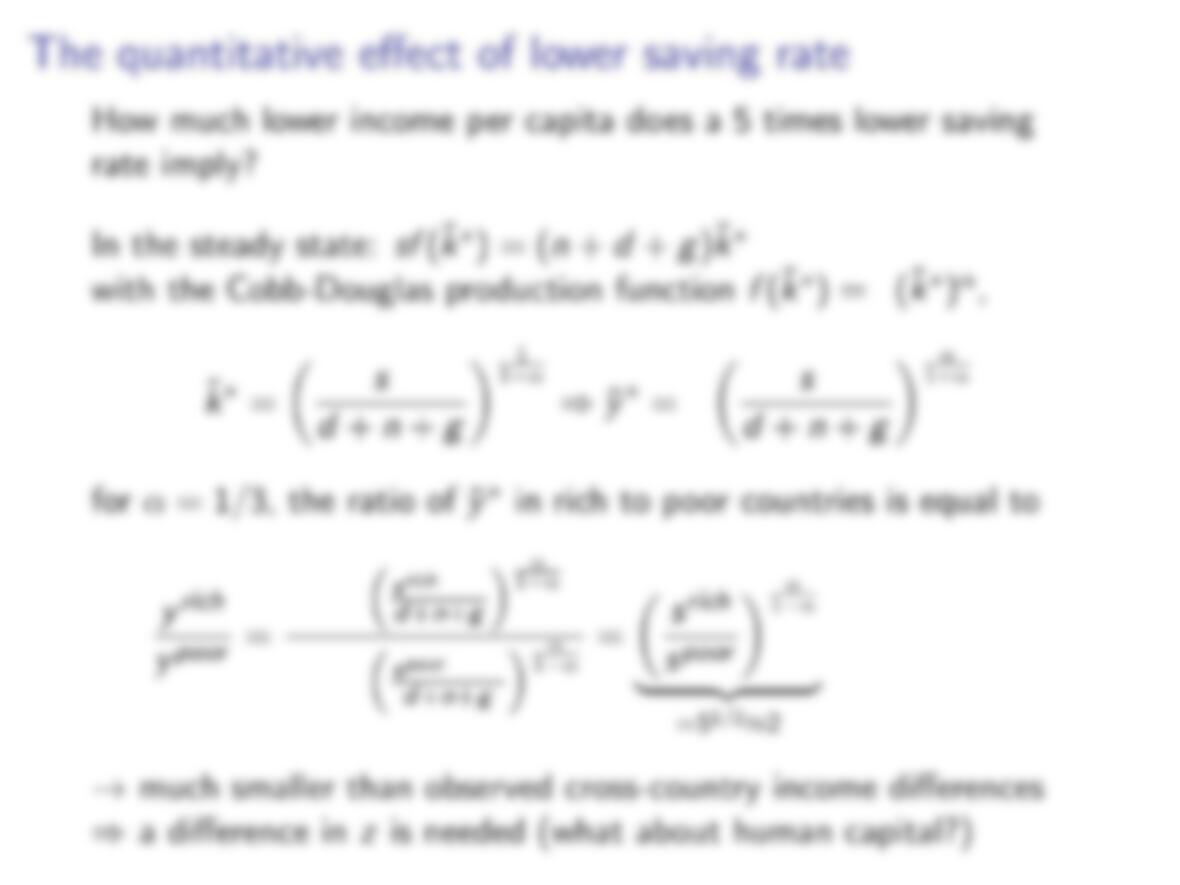
→much smaller than observed cross-country income differences

sAk
sAk
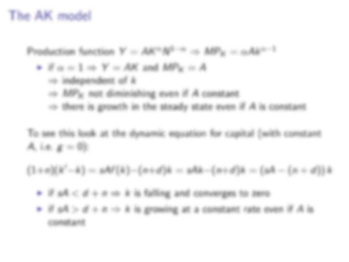
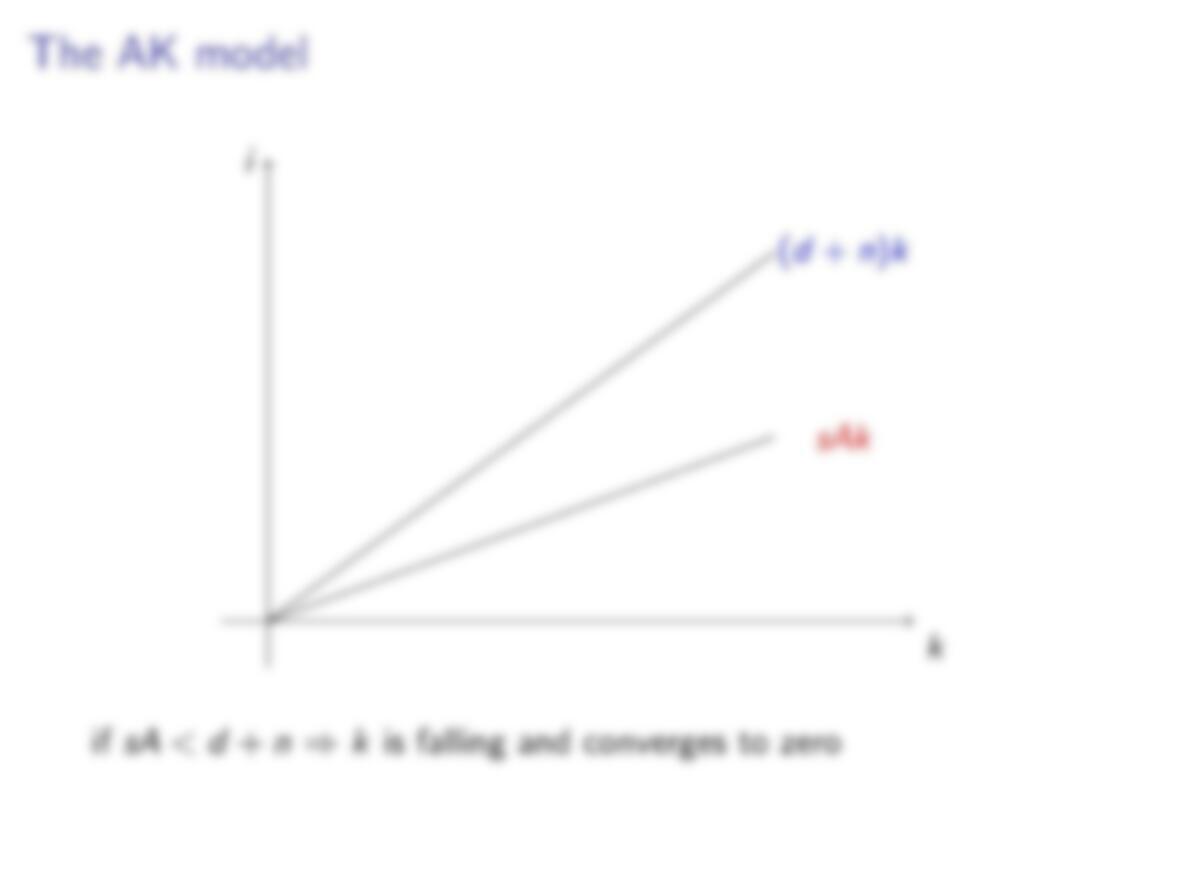
if sA <d+n⇒kis falling and converges to zero
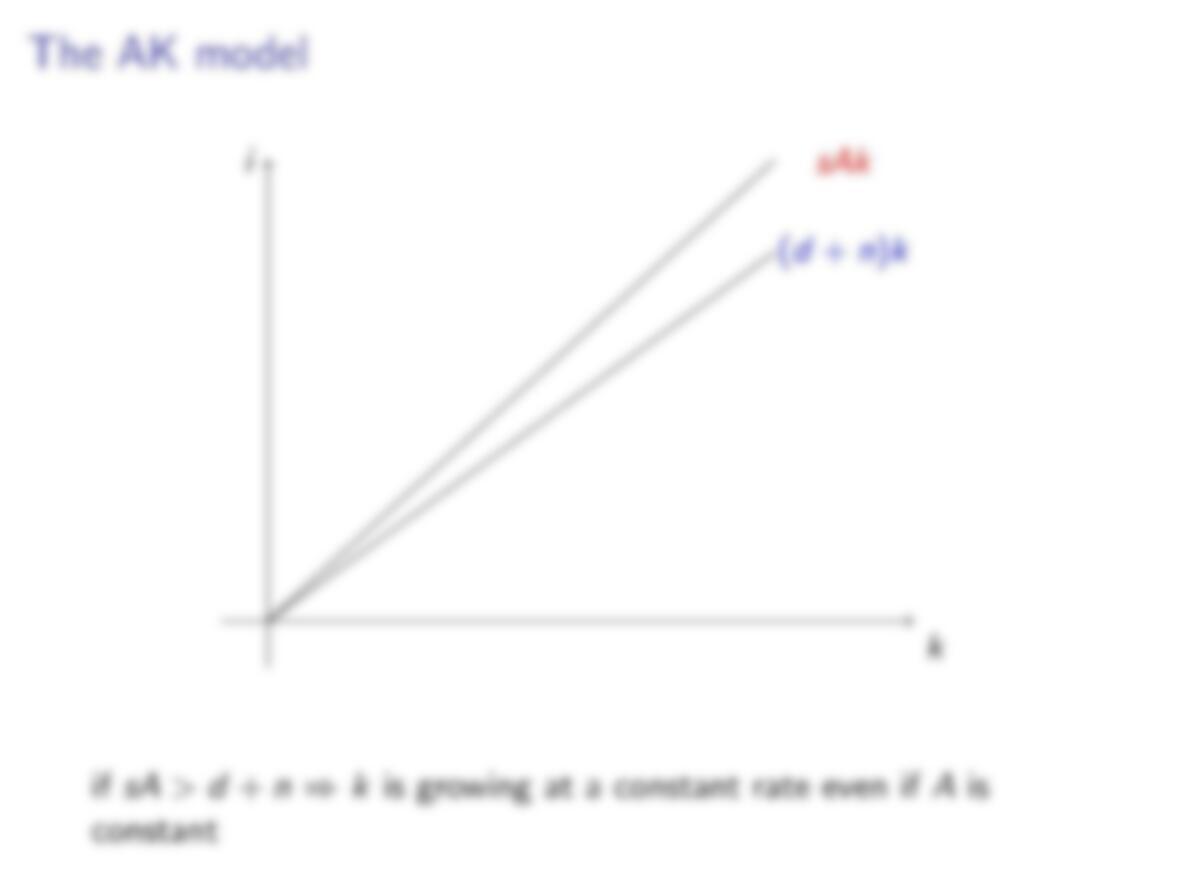
if sA >d+n⇒kis growing at a constant rate even if Ais
constant
sAk
if sA >d+n⇒kis growing at a constant rate even if Ais
constant
sAk
if sA <d+n⇒kis falling and converges to zero