Demand & Business
Forecasting
Assignment
By
Anshuman Prakash
Roll No: B11070
Study of Bivariate & Multiple Linear Regression & Applying both the Models to the chosen Variables to
understand the relationship between them and fit a suitable Model .The variables chosen for the
analysis are GDP as the dependent variable & Capital Formation, Labor Force & FDI as the independent
variable. The study has been done on the countries India, China & Brazil to study the impact of the
various factors on GDP growth from 1992-2008.

Anshuman Prakash B11070
Contents
Executive Summary: …………………………………………………………………………………………………………………….. 3
Bi-Variate Series ………………………………………………………………………………………………………………………….. 4
Scatter Plot & Various Functional Forms …………………………………………………………………………………….. 4
Scatter Plot ………………………………………………………………………………………………………………………….. 4
Functional Forms: ………………………………………………………………………………………………………………... 4
Linear: GDP=β0 + β1FDI ………………………………………………………………………………………………………. 5
Quadratic: GDP=β0 + β1*FDI+β2*(FDI^2) ……………………………………………………………………………. 6
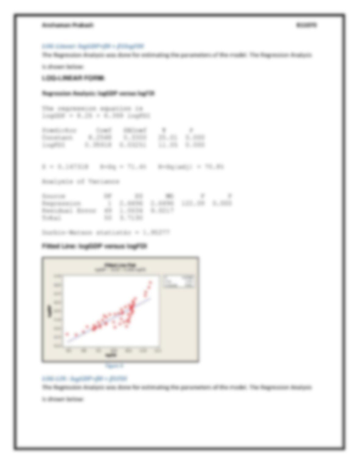
LOG-Linear: logGDP=β0 + β1logFDI …………………………………………………………………………………….. 7
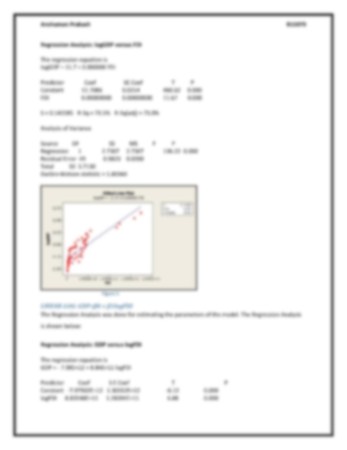
LOG-LIN : logGDP=β0 + β1FDI …………………………………………………………………………………………….. 7
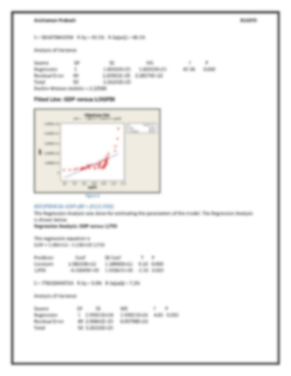
LINEAR-LOG: GDP=β0 + β1logFDI………………………………………………………………………………………… 8
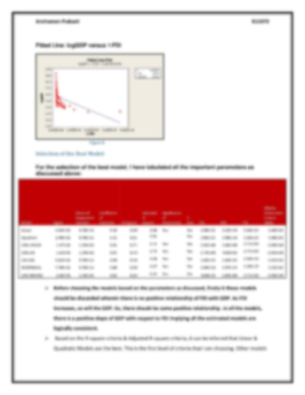
RECIPROCAL-GDP=β0 + β1(1/FDI) ……………………………………………………………………………………….. 9
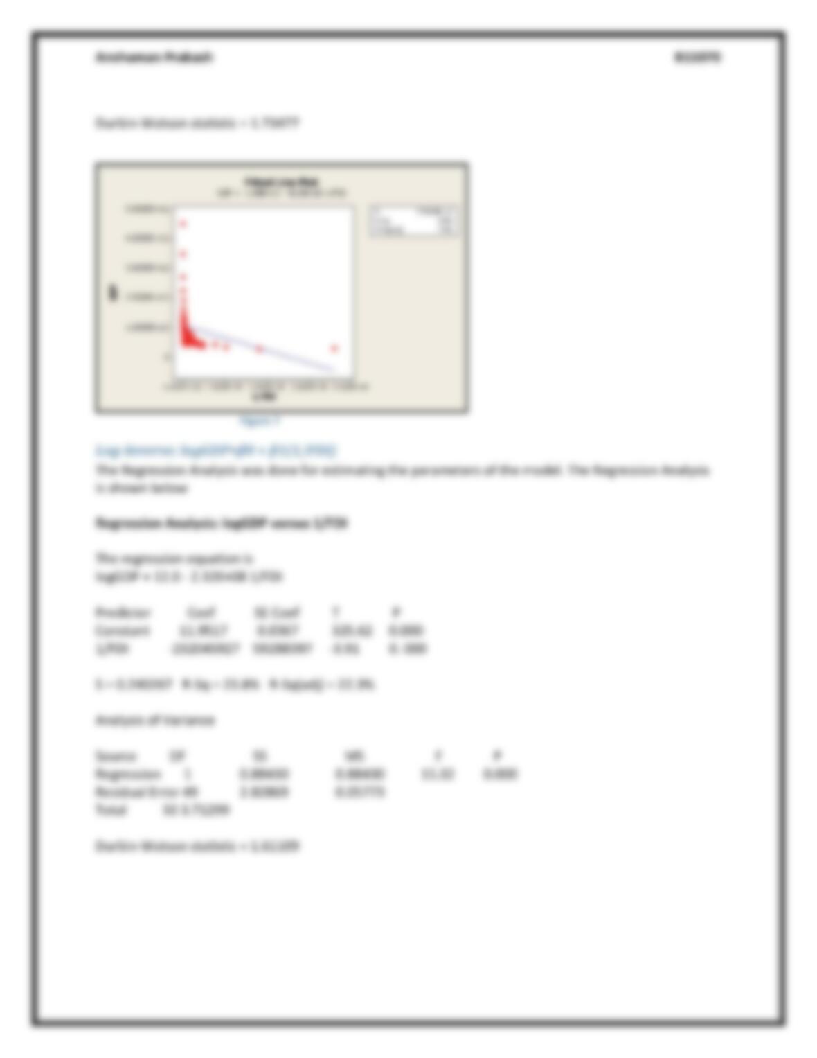
Log-Inverse: logGDP=β0 + β1(1/FDI) ………………………………………………………………………………….. 10
Selection of the Best Model: ………………………………………………………………………………………………… 11
Interpretation of the Estimated Regression Model …………………………………………………………………. 12
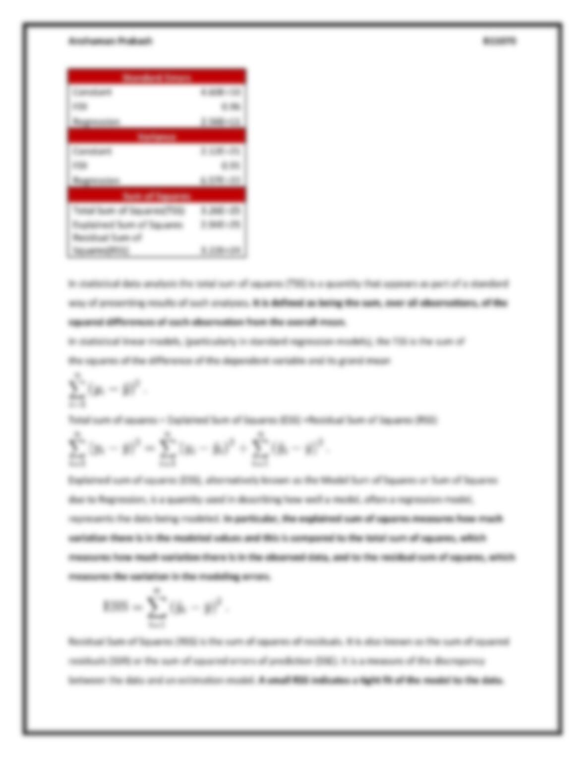
Standard Errors, TSS, ESS & RSS ……………………………………………………………………………………………….. 12
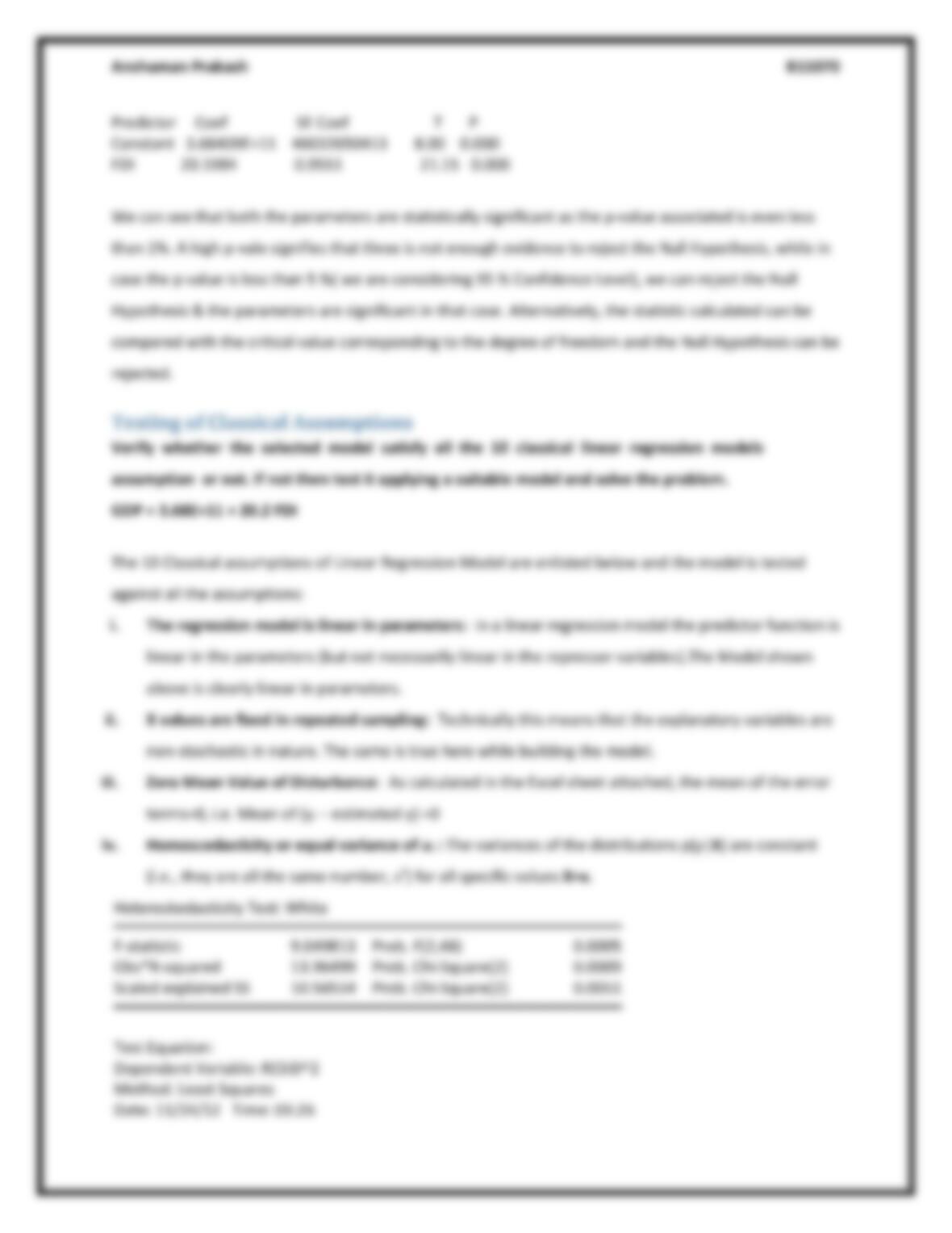
Hypothesis Testing of the Parameters ………………………………………………………………………………………. 14
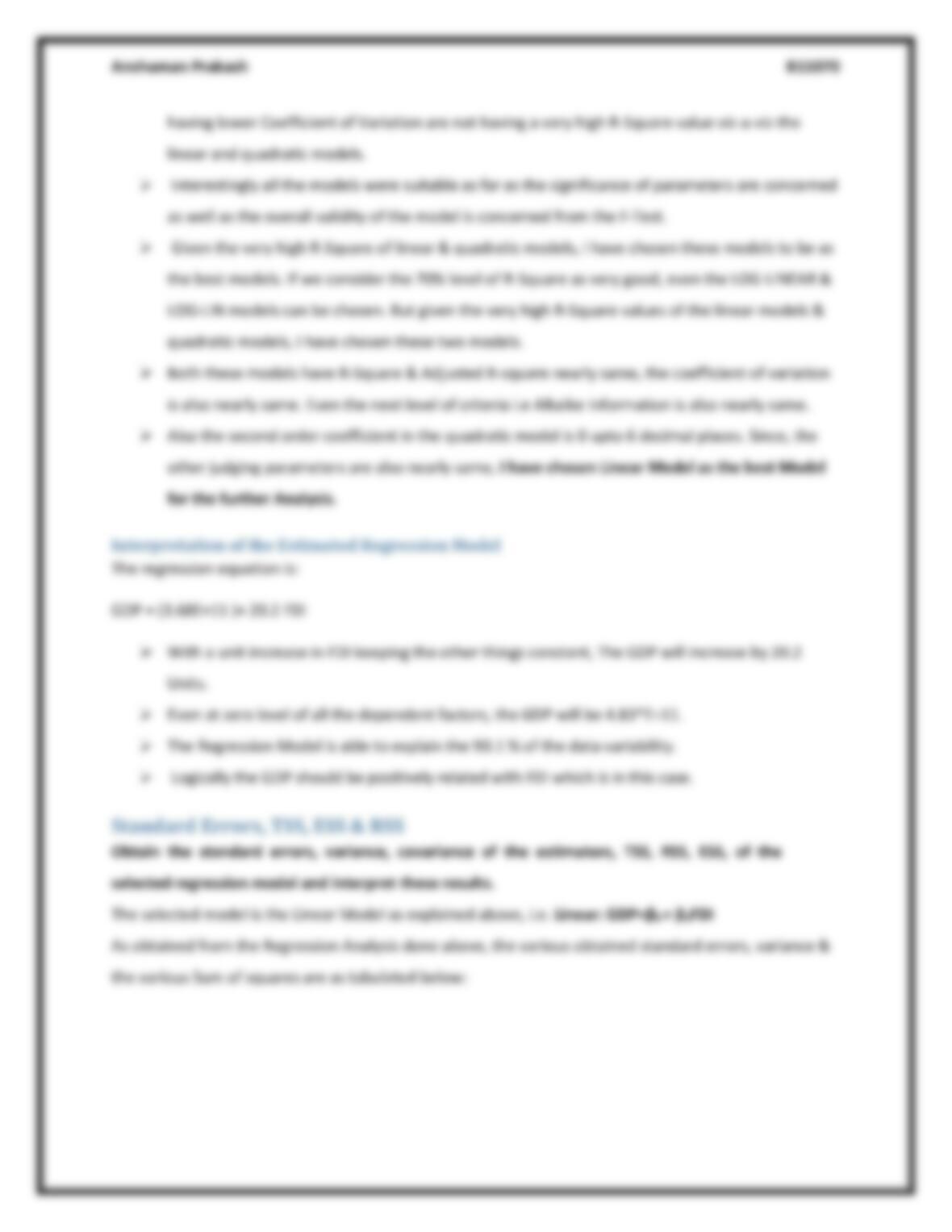
Testing of Classical Assumptions ……………………………………………………………………………………………… 15
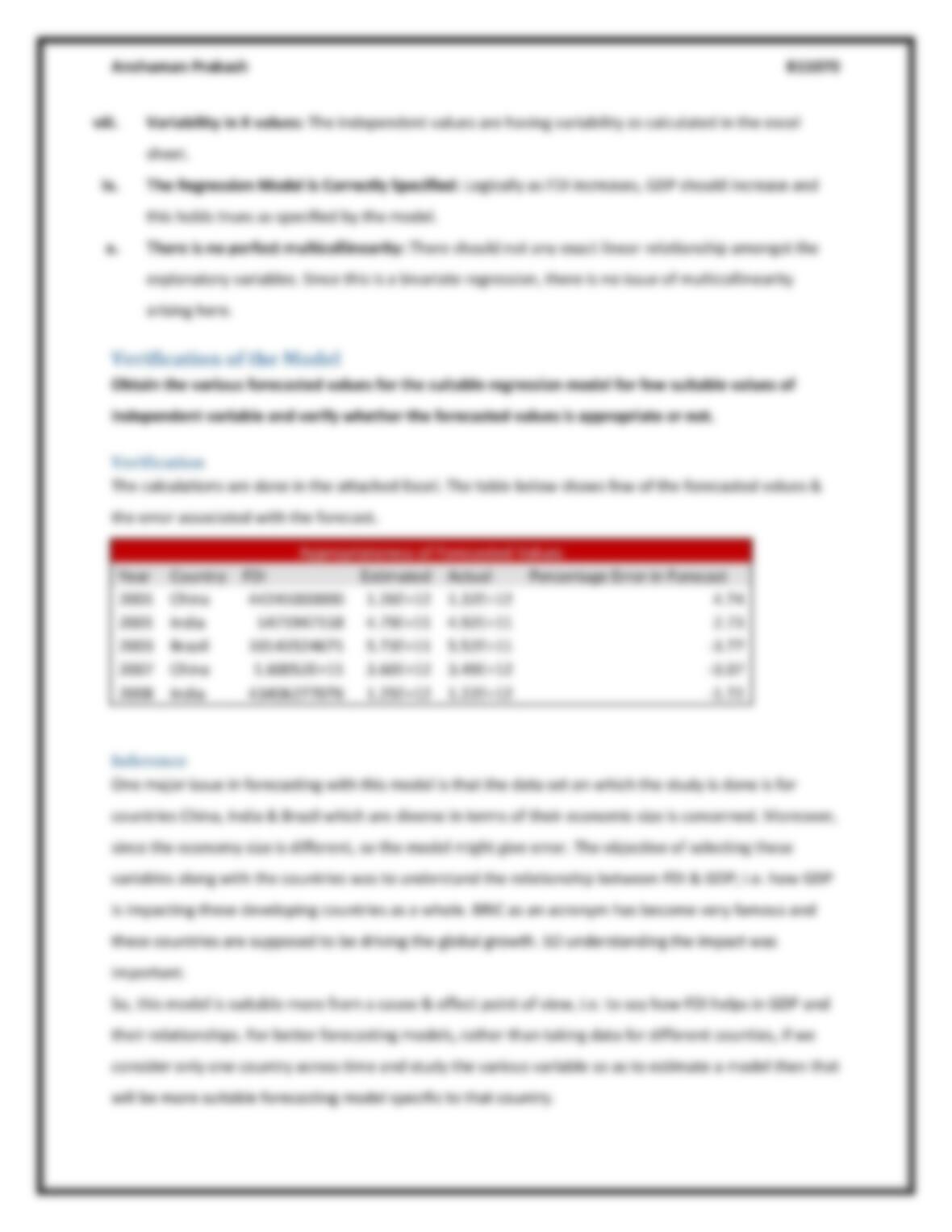
Verification of the Model ………………………………………………………………………………………………………… 18
Verification ………………………………………………………………………………………………………………………… 18
Inference …………………………………………………………………………………………………………………………… 18
Multivariate Series ……………………………………………………….……………………………………………………………. 19
Multiple Linear Regressions & Testing of Hypothesis: ………………………………………………………………… 19
Multiple Linear Regression ………………………………………………………………………………………………….. 19
Interpretation of the Estimated Regression Model …………………………………………………………………. 20
Hypothesis Testing of the Parameters …………………………………………………………………………………… 21
t-tests …………………………..……………………………………………………………………………………………….. 21
F-Test …………………………………………………………………………………………………………………………….. 22
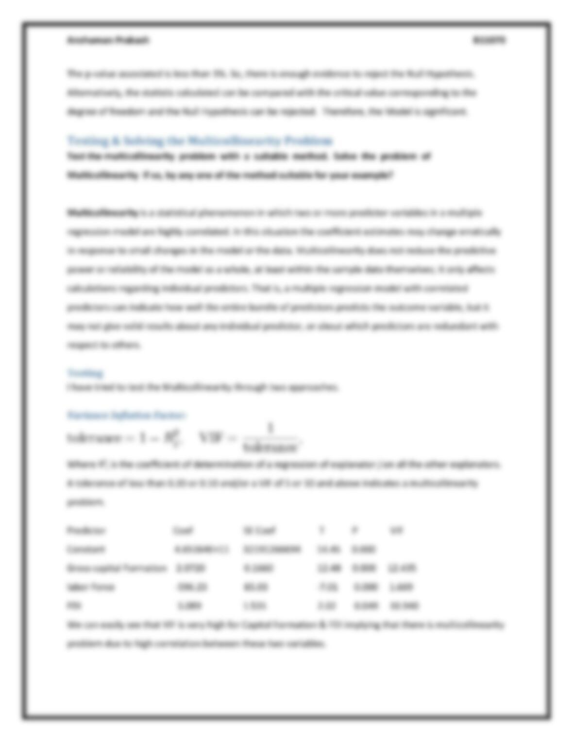
Testing & Solving the Multicollinearity Problem ………………………………………………………………………… 23
Testing ………………………………………………………………………………………………………………………………. 23
Variance Inflation Factor: …………………………………………………………………………………………………. 23
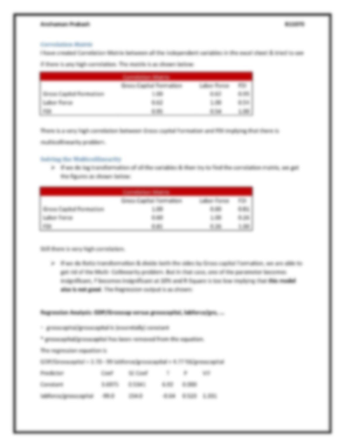
Correlation Matrix …………………………………………………………………………………………………………… 24

Anshuman Prakash B11070
Solving the Multicollinearity ………………………………………………………………………………………………… 24
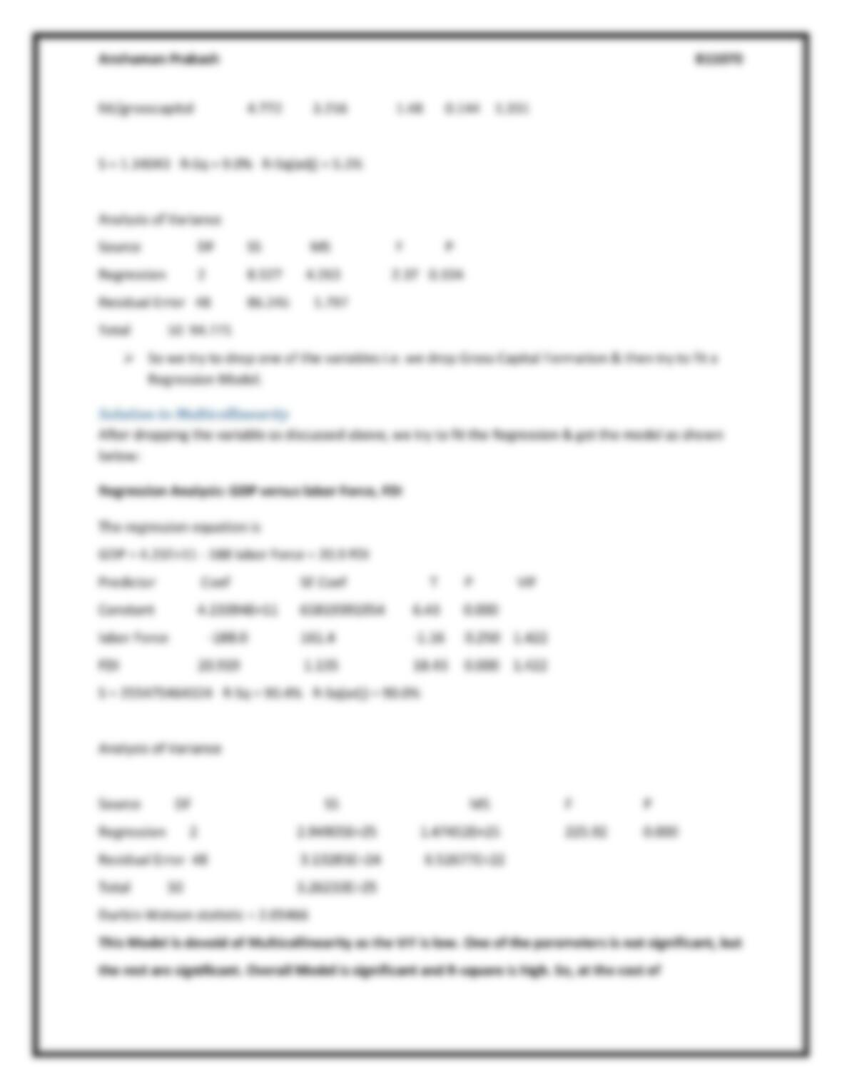
Solution to Multicollinearity …………………………………………………………………………………………….. 25
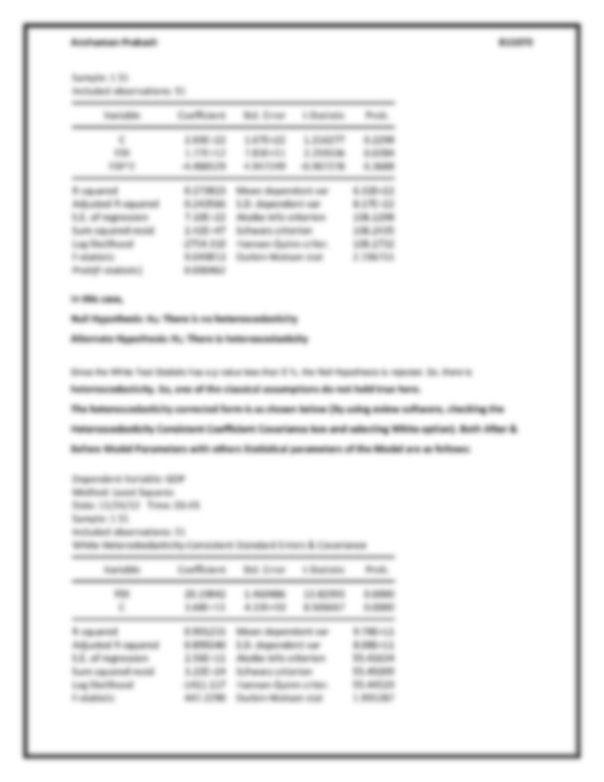
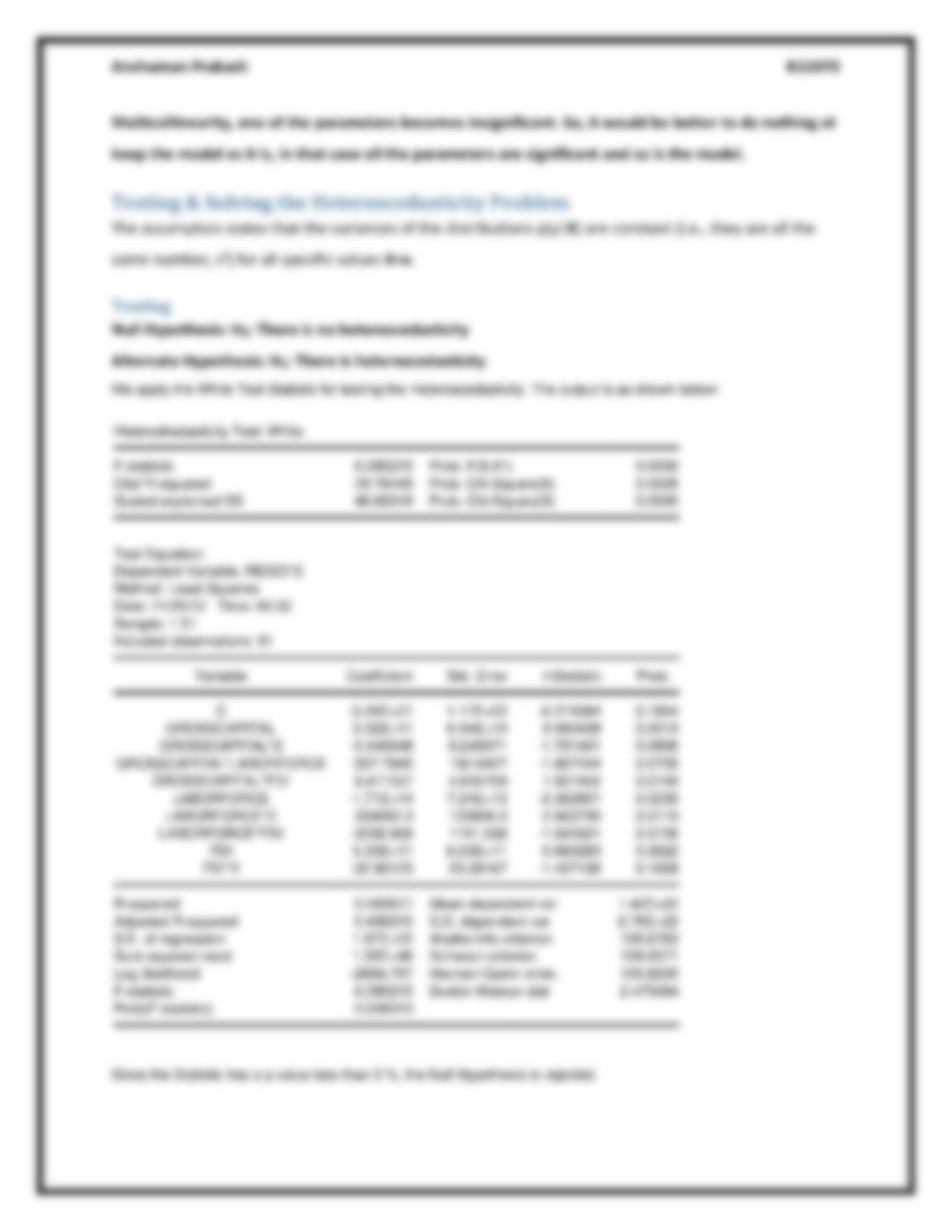
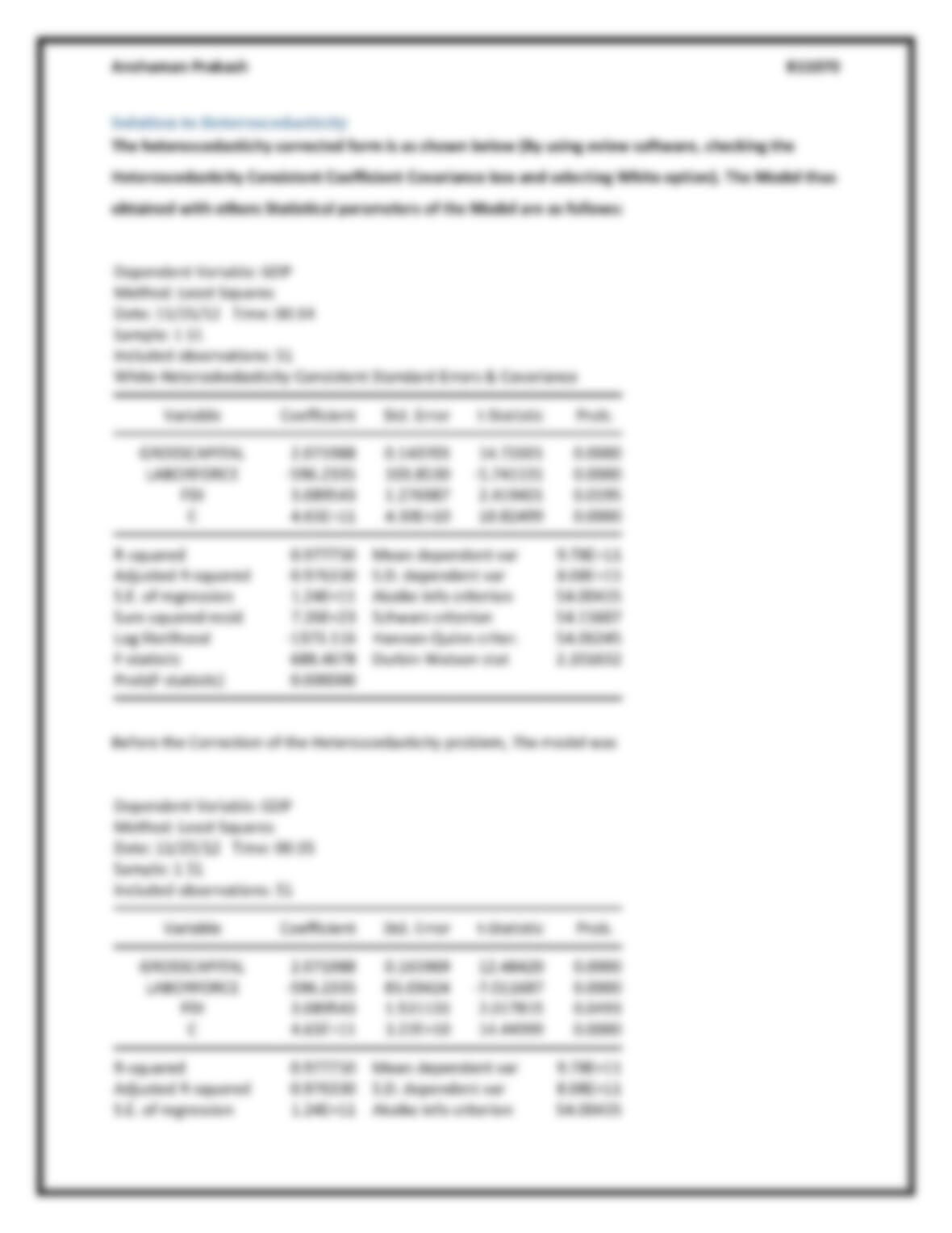
Testing & Solving the Heteroscedasticity Problem ……………………………………………………………………… 26
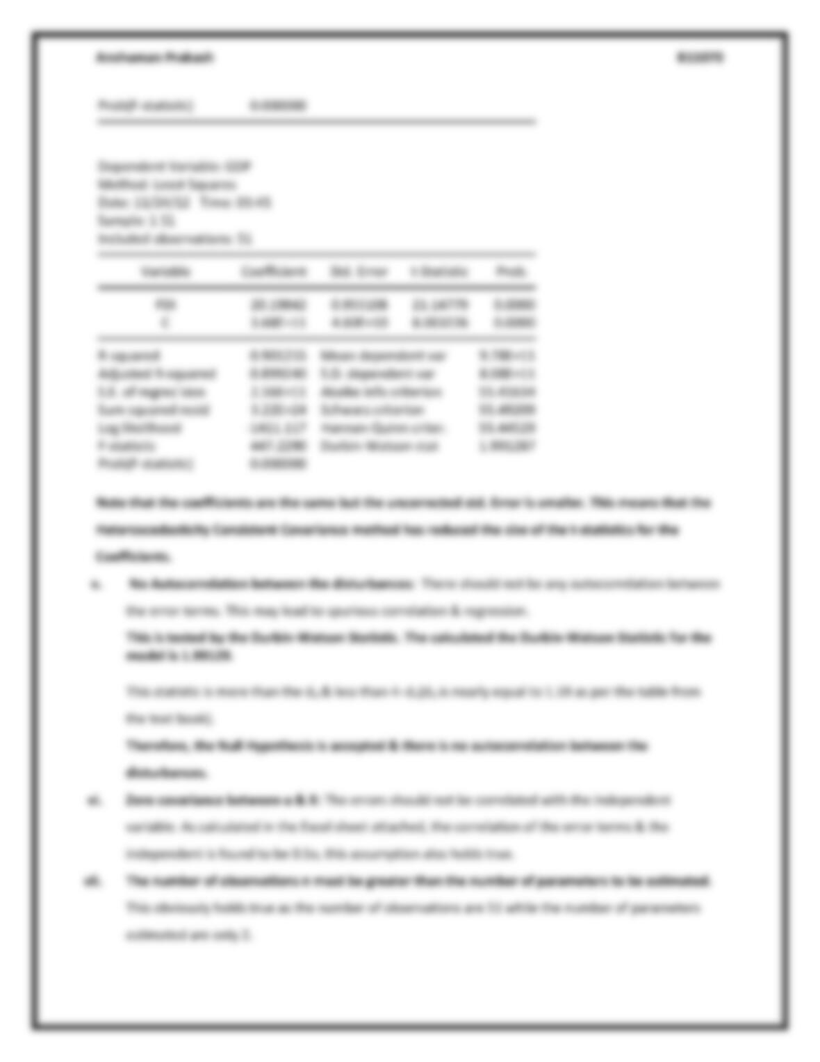
Testing ………………………………………………………………………………………………………………………………. 26
Solution to Heteroscedasticity ……………………………………………………………………………………………… 27
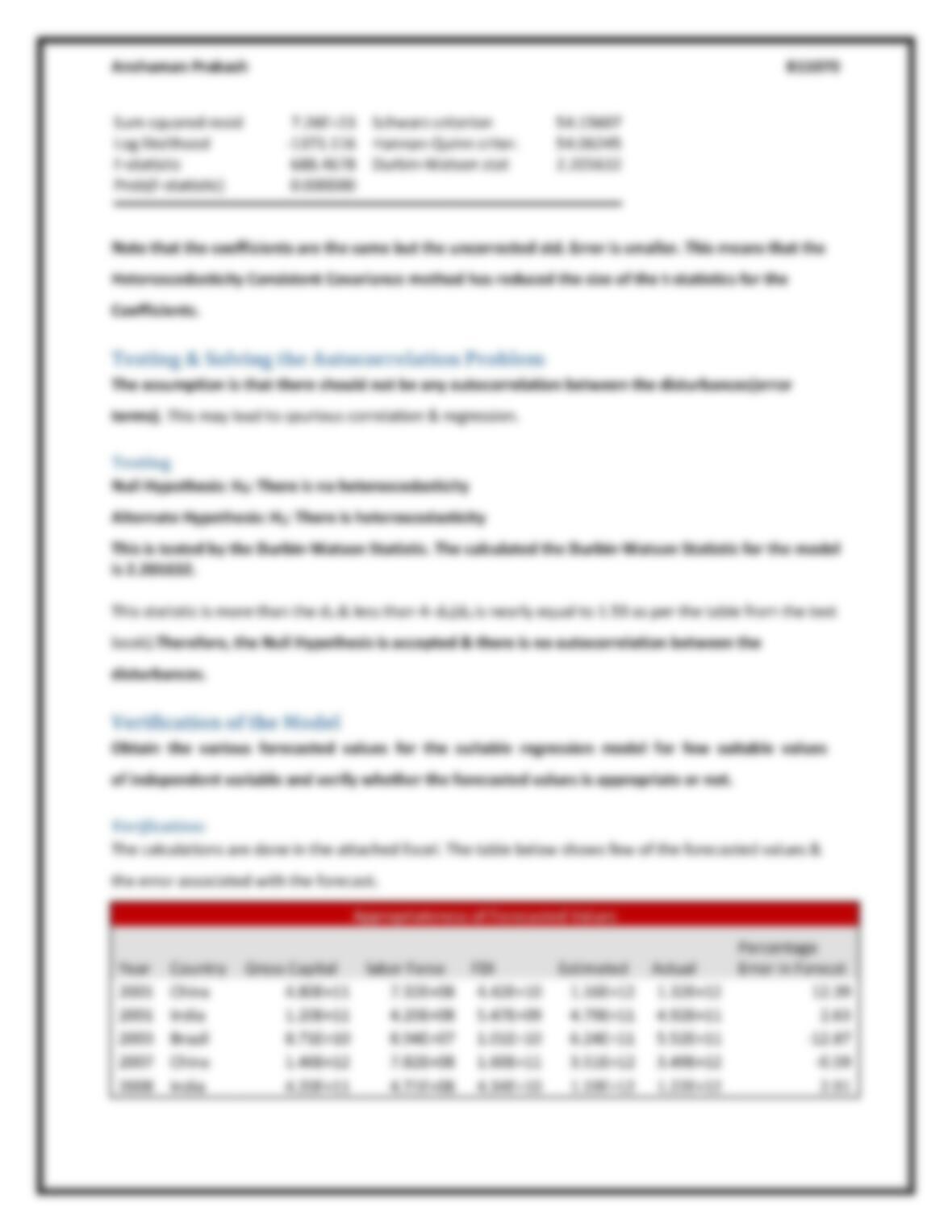
Testing & Solving the Autocorrelation Problem …………………………..…………………………………………….. 28
Testing ………………………………………………………………………………………………………………………………. 28
Verification of the Model ………………………………………………………………………………………………………… 28
Verification: ……………………………………………………………………………………………………………………. 28
Inference: ………………………………………………………………………………………………………………………. 29
Figure 1 ……………………………………………………………………………………………………………………………………… 4
Figure 2 ……………………………………………………………………………………………………………………………………… 6
Figure 3 ……………………………………………………………………………………………………………………………………… 6
Figure 4 ……………………………………………………………………………………………………………………………………… 7
Figure 5 ……………………………………………………………………………………………………………………………………… 8
Figure 6 ……………………………………………………………………………………………………………………………………… 9
Figure 7 ……………………………………………………………………………………………………………………………………. 10
Figure 8 ……………………………………………………………………………………………………………………………………. 11

Anshuman Prakash B11070
Executive Summary:
The general purpose of multiple regressions is to learn more about the relationship between several
independent or predictor variables and a dependent or criterion variable. I have chosen following
variables for the assignment.
Y= β0+ β1(K)+ β2(L)+ β3(FDI)+error
Y
Gross Domestic Product
K
Gross Capital Formation
L
Labor Force
FDI
Foreign Direct Investment
Since the data for Human Capital was not available, I exclude that variable from the Model. The
objective was to understand the relationship of these variables in determining the GDP and the same
was done by taking the data of China, Brazil & India from 1992-2008
.
The Bivariate as well as Multivariate Analysis has been done as the part of the project for creating a
model. One major issue in forecasting with this model is that the data set on which the study is done is
for countries China, India & Brazil which are diverse in terms of their economic size is concerned.
Moreover, since the economy size is different, so the model might give error. The objective of selecting
these variables along with the countries was to understand the relationship between FDI & GDP; i.e.
how GDP is impacting these developing countries as a whole. BRIC as an acronym has become very
famous and these countries are supposed to be driving the global growth. SO understanding the impact
was important.
So, this model is suitable more from a cause & effect point of view, i.e. to say how FDI helps in GDP and
their relationships. For better forecasting models, rather than taking data for different counties, if we
consider only one country across time and study the various variable so as to estimate a model then that
will be more suitable forecasting model specific to that country.
The data set has been collected from the databank of World Bank. The databank from World Bank offers
various data arrangement tools, as a result required data can be arranged in desired format and direct
exel file can be downloaded. The data set consists of GDP(PPP) in current international US Dollars in
millions, FDI inflow (as % of GDP), Gross Capital Formation (as % of GDP), Labor Force .
Anshuman Prakash B11070
Assignment
Bi-Variate Series
Scatter Plot & Various Functional Forms
Plot the data in a scatter form, specify and estimate the various functional form of regression
model, select the best model among them and interpret the results of the estimates regression
model.
Scatter Plot
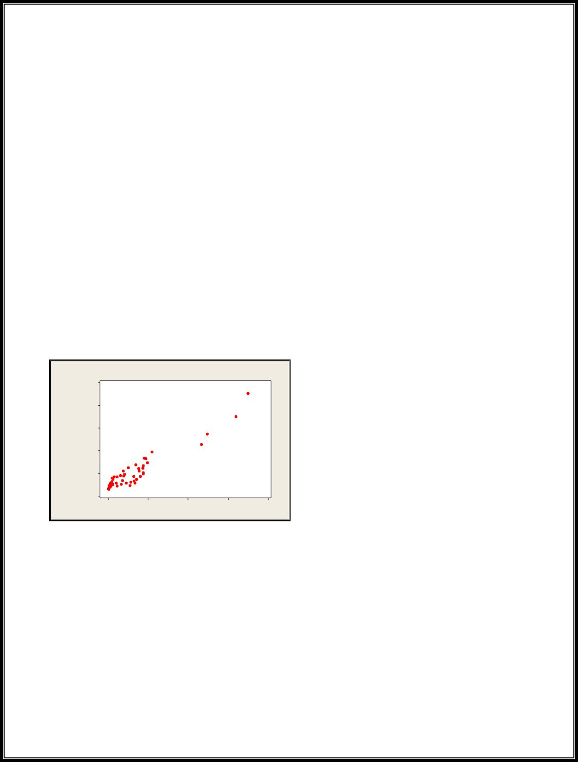
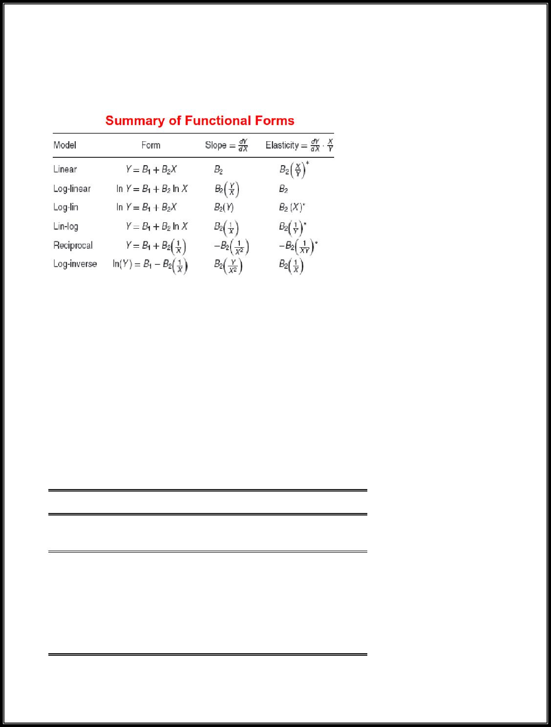
The variables that I have chosen for the analysis are GDP as the dependent variable & FDI as the
independent variable. The study has been done on the countries India, China & Brazil to study the
impact of FDI on GDP growth. The data has been collected from 1992 to 2008 for building up the model
& then the available data points are used to validate the model in terms of the forecasting error with
respect to the data available viz a viz the forecasted value. The Fig. 1 below shows the scatter plot of the
variates.
2.0000E+111.5000E+111.0000E+115.0000E+100
5.0000E+12
4.0000E+12
3.0000E+12
2.0000E+12
1.0000E+12
0
FDI
GDP
Scatterplot of GDP vs FDI
Figure 1
Functional Forms:
We can see from the scatter plot that there seems to be a relationship between both the variables
chosen. For better understanding the exact nature of relationship, I have tried to use various functional
forms as discussed below and tried to choose the best of them on the basis of few parameters like:
➢ R-Square
➢ Adjusted R-Square
➢ Alkaike Information Criterion in case of close values of R-Square & Adjusted R-Square
➢ Coefficient of Variation.
Anshuman Prakash B11070
All these comparisons make sense only if the parameters of the model are statistically significant as well
as the Model as a whole is statistically significant. This emphasizes the importance of t-tests and F-test.
The various functional forms that I have tried to estimate are:
The various functional forms have been estimated & discussed below:
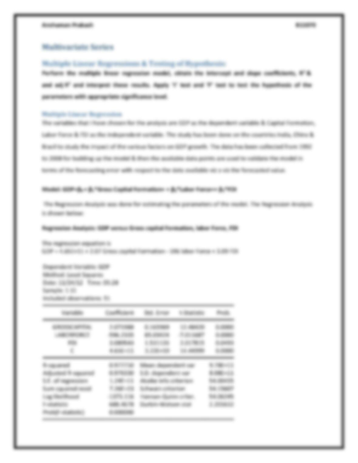
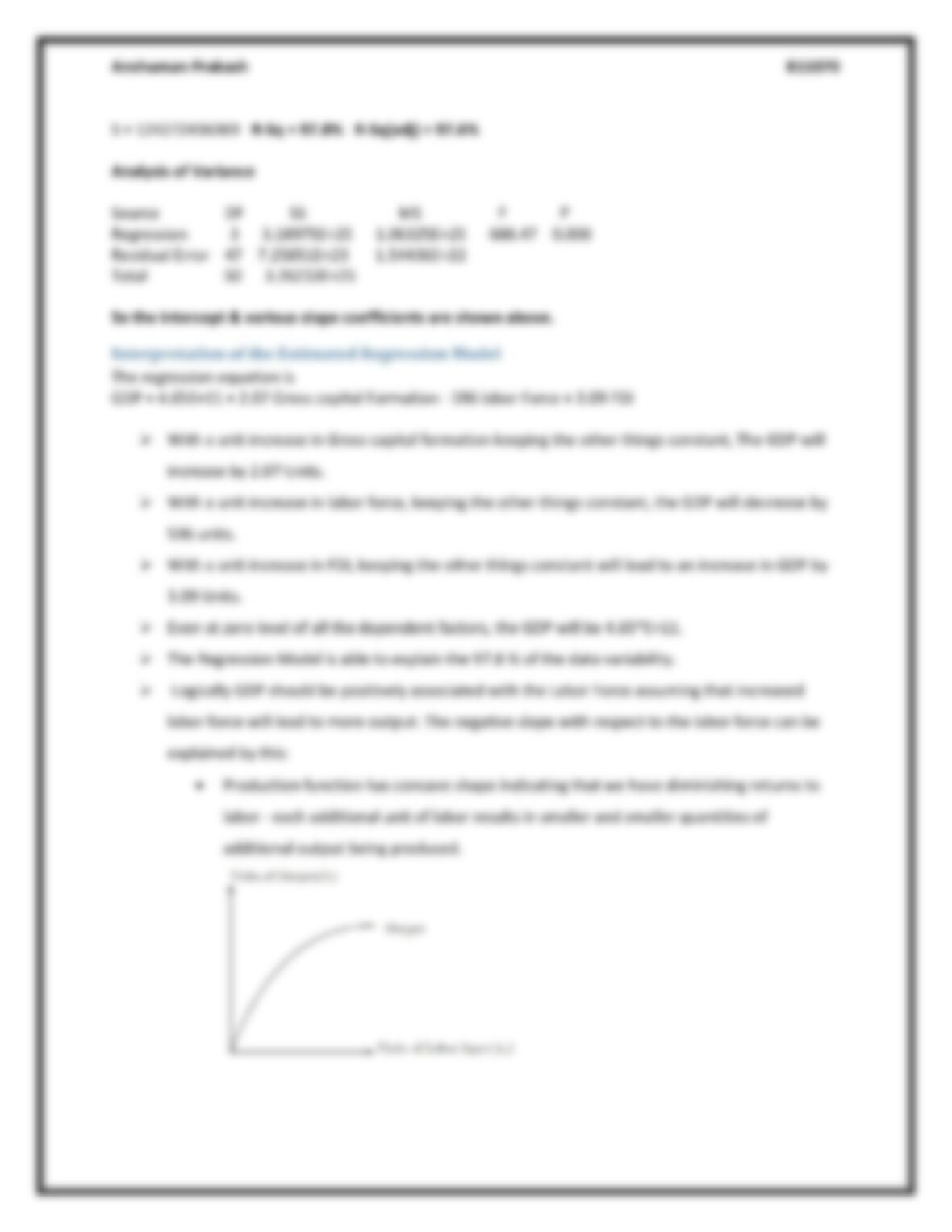
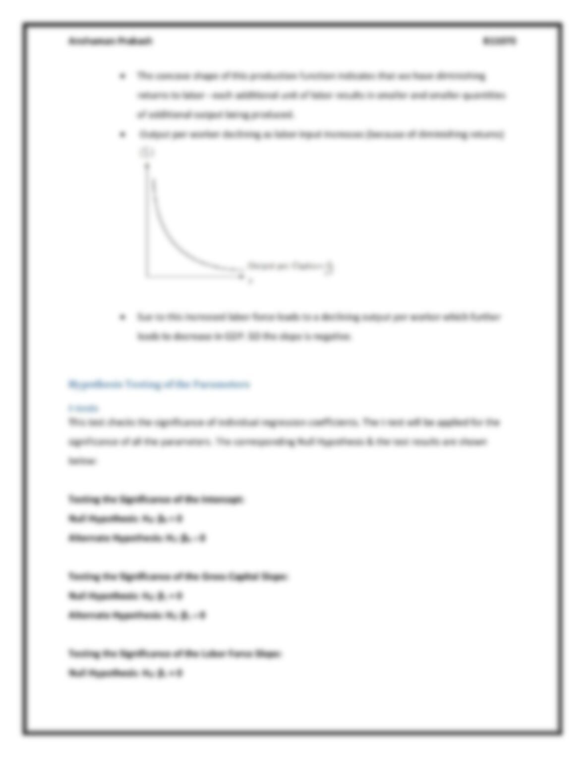
Linear: GDP=β0 + β1FDI
The Regression Analysis was done for estimating the parameters of the model. The Regression Analysis
is shown below:
Regression Analysis: GDP versus FDI
The regression equation is
GDP = 3.68E+11 + 20.2 FDI
Dependent Variable: GDP
Method: Least Squares
Date: 11/23/12 Time: 19:35
Sample: 1 51
Included observations: 51
Variable
Coefficient
Std. Error
t-Statistic
Prob.
FDI
20.19842
0.955108
21.14779
0.0000
C
3.68E+11
4.60E+10
8.003226
0.0000
R-squared
0.901255
Mean dependent var
9.78E+11
Adjusted R-squared
0.899240
S.D. dependent var
8.08E+11
S.E. of regression
2.56E+11
Akaike info criterion
55.41634
Sum squared resid
3.22E+24
Schwarz criterion
55.49209
Log likelihood
-1411.117
Hannan-Quinn criter.
55.44529
F-statistic
447.2290
Durbin-Watson stat
1.991287
Prob(F-statistic)
0.000000
Anshuman Prakash B11070
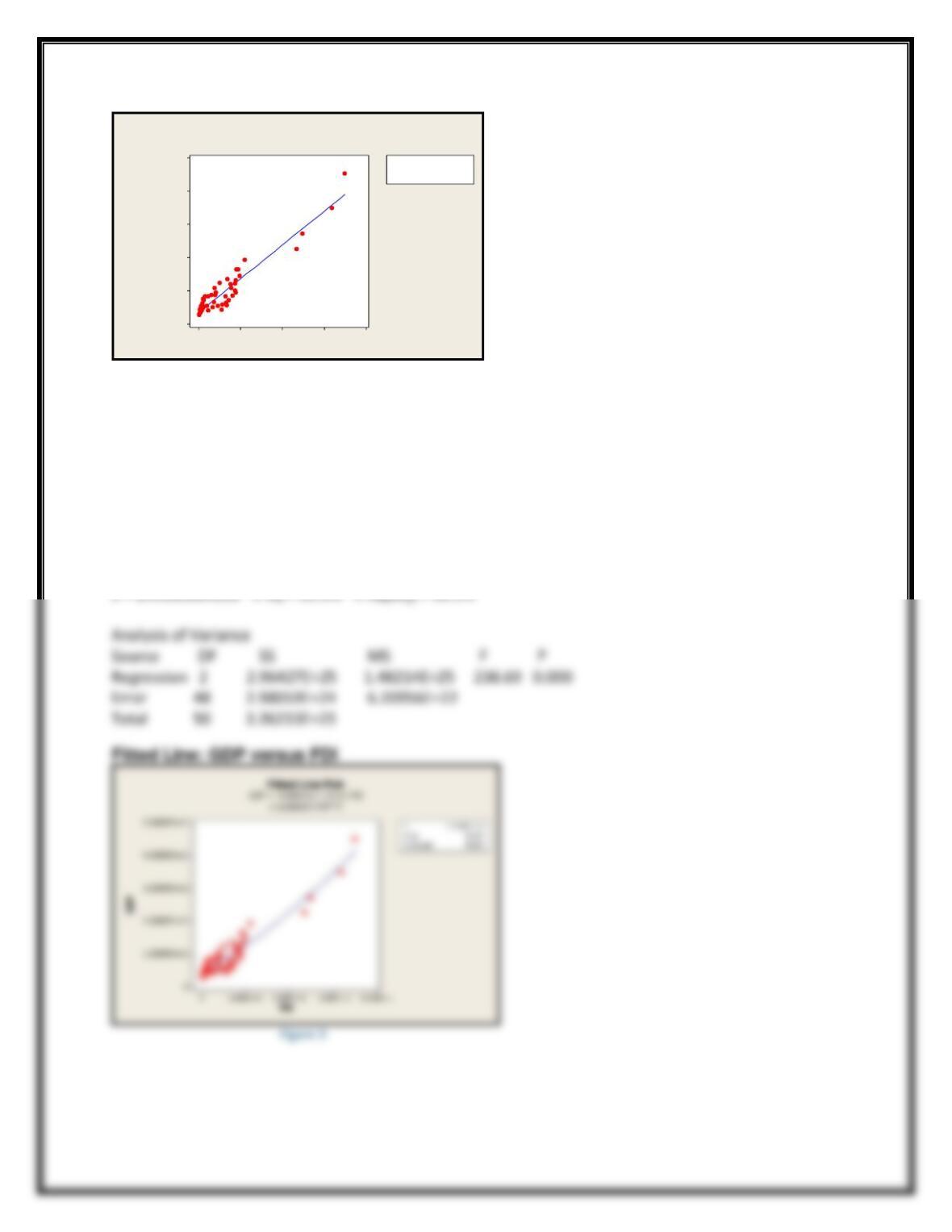
2.0000E+111.5000E+111.0000E+115.0000E+100
5.0000E+12
4.0000E+12
3.0000E+12
2.0000E+12
1.0000E+12
0
FDI
GDP
S 2.56404E+11
R-Sq 90.1%
R-Sq(adj) 89.9%
Fitted Line Plot
GDP = 3.68E+11 + 20.20 FDI
Figure 2
Quadratic: GDP=β0 + β1*FDI+β2*(FDI^2)
The Regression Analysis was done for estimating the parameters of the model. The Regression Analysis
is shown below:
Polynomial Regression Analysis: GDP versus FDI
The regression equation is
GDP = 4.42E+11 + 15.11 FDI + 0.000000 FDI**2