DEMAND ANALYSIS AND OPTIMAL PRICING
INTENDED LEARNING OUTCOMES
1. State the law of demand and its determinants.
3. Apply the principles of elasticities in managerial decision-making.
4. Apply the value of elasticities and total revenue in determining optimal prices in the market.
5. Use optimal pricing strategy in solving managerial decision-making problems.
6. Explain price discrimination by providing real-life examples.
In this chapter, we will take a closer look at demand and the role it plays in managerial
decision making. We begin this chapter by considering the multiple determinants of demand. Next,
we look more closely at the responsiveness of demand to these factors, a concept captured in the
basic definition of elasticity. In the remaining sections, we present a richer formulation of demand
and show how it can be used to guide managers in their goal of maximizing profits. Toward this end,
we will refine our optimization techniques to account for more complicated demand conditions—
those that include the possibilities of market segmentation and price discrimination.
THE DEMAND FUNCTION
Demand function shows the relationship between the quantity sold of a good or service and
one or more variables. 𝐐 = 𝐟(𝐱′𝐬)
Where: Q = quantity sold of a good/service
x’s = determinants of demand
Suppose that 𝐐 = 𝐟(𝐏, 𝐏𝐎,𝐘)
Where: P = price of a good/service
PO= price of related good/service
Y = income
Example: Given the demand for air travel
Q = 25 + 3Y + PO – 2P
Where: Q = number of airline’s coach seats sold per flight
P = airline’s coach fare
PO = competitor’s price
Y = income in the region
Currently your airline and your competitor are charging the same one-way fare, $240. The
current level of income in the region is 105.
We find that
Q = 25 + 3(105) + 1(240) – 2(240) = 100 seats
• The demand equation can be used to test the effect of changes in any of the explanatory
variables. From Equation we see that
3
1. For each point increase in the income index, 3 additional seats will be sold.
2. For each $1 increase in the airline’s fare, 2 fewer seats will be sold.
3. For each $1 increase in the competitor’s fare, 1 additional seats will be sold.
Each of these results assumes the only change that occurs; that is, all other factors are held
constant. In fact, the total change in demand caused by simultaneous changes in the explanatory
variables can be expressed as:
∆Q = 3∆Y + 1∆PO – 2∆P
• Thus, if income increases by 5 index points while both airline prices are cut by $15, we find
∆Q = 3(5) + 1(-15) – 2(–15) = 30 seats. Your airline would expect to sell 30 additional seats on
each flight.
The Demand Curve and Shifting Demand
• Suppose that in the future that the regional income (Y) = 105 and the competitor’s fare (PO)
= $240. However, your airline’s fare (P) is not set in stone, and you are interested in testing
the effect of different possible coach prices.
• Substituting the values of Y and PO into demand function, we find that
Q = 25 + 3(105) + 1(240) – 2P
Q = 580 – 2P (movement along the demand curve)
• The equation relates the quantity of the good or service sold to its price, holding all other
factors affecting demand constant (Y and PO)
• We can graph this demand equation as demand curve that describes a downward sloping
curve.
The Demand Curve and Shifting Demand
• But what happens if there is a change in one of the other factors that affect demand? Such a
change causes a shift in the demand curve.
• Suppose that a year from now P is expected to be unchanged but Y is forecast to grow to
119. What will the demand curve look like a year hence?
• Substitute the new value, Y = 119 (along with P = 240), into the demand function to obtain
Q = 25 + 3(119) + 1(240) – 2P
Q = 622 – 2P (shift the demand curve)
The Demand Curve and Shifting Demand
Q = 580 – 2P or P = 311 – Q/2
Q = 622 – 2P or P = 290 – Q/2
• The constant term of the new demand curve is larger than that of the old. The figure
underscores this point by graphing both the old and new demand curves.
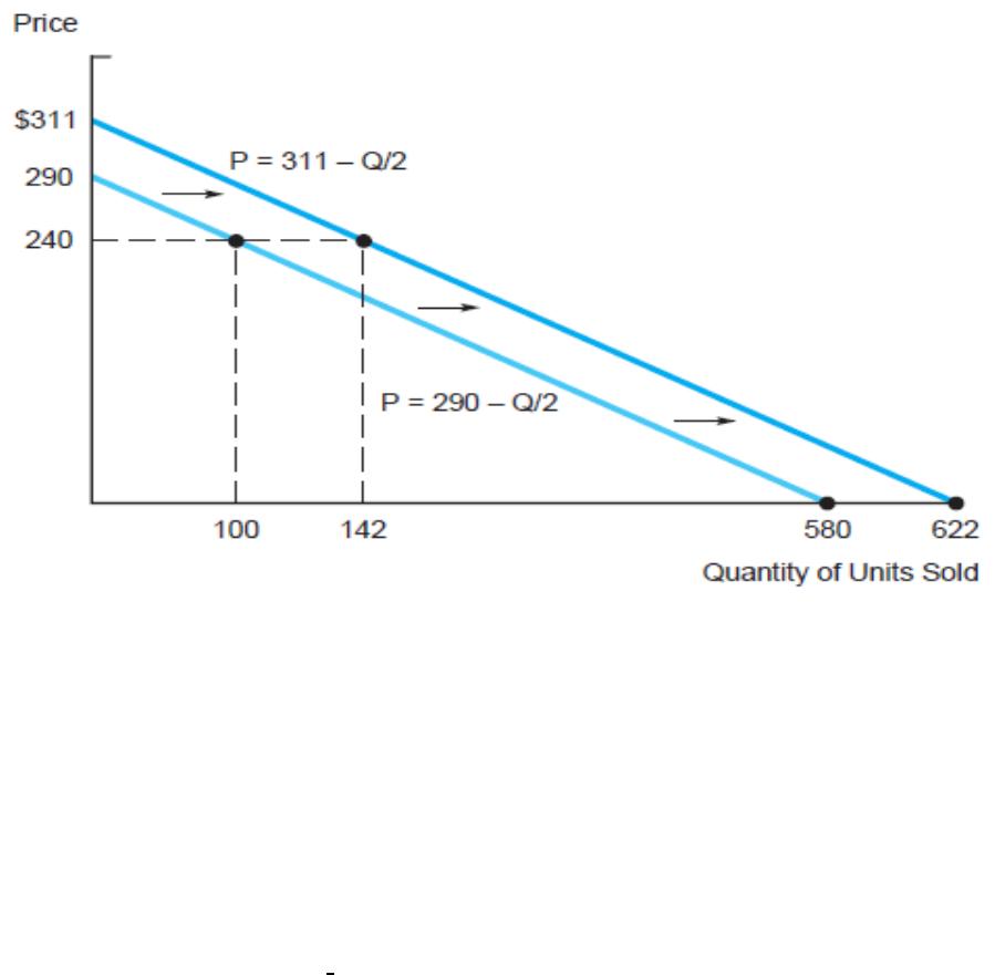
Figure 4.1 The Demand Curve Shifting.
• The new demand curve constitutes a parallel shift to the right (toward greater sales
quantities) of the old demand curve.
• At P $240, current demand is 100 seats per flight. At the same fare, coach demand one year
from now is forecast to be 142 seats (due to the increase in regional income), a gain of 42
seats.
Q = 580 – 2P = 580 – 2(240) = 100
Q = 622 – 2P = 622 – 2(240) = 142
GENERAL DETERMINANTS OF DEMAND
• Good’s own price (P) is the key determinant of demand
• Other determinants of demand:
1. Level of income (Y) of the potential purchasers of the good or service.
a. Normal good – a good in which an increase in income raises its sales.
b. Inferior good – a good in which an increase in income causes a reduction in spending.
2. Prices of related goods
a. Substitute good – a good in which can substitute for another good (competitor’s
good). An increase in the price of the substitute good or service causes an increase in
demand for the another good.
b. Complementary good – a good that complements with another good. That is, an
increase in demand for one causes an increase in demand for the other. An increase
in the price of a complementary good reduces demand for the another good.
3. Population (number of consumers that consume goods/services)
4. Tastes and preferences
5. Consumer’s expectation towards future market condition (future price, product
availability and future income)
ELASTICITY OF DEMAND
• Price elasticity measures the responsiveness of a good’s sales to changes in its price.
• Price elasticity of demand is the ratio of the percentage change in quantity and the
percentage change in the good’s price, all other factors held constant.
𝐄𝐏=%∆𝐐
%∆𝐏
• Point elasticity formula:
𝑬𝑷=∆𝐐
𝐐𝐱 𝟏𝟎𝟎
∆𝐏
𝐏𝐱𝟏𝟎𝟎 =(𝐐𝟏−𝐐𝟎)
𝐐𝟎
(𝐏𝟏−𝐏𝟎)
𝐏𝟎
• For example, consider the airline’s demand curve as described in equation. At the current
fare of $240, 100 coach seats are sold. If the airline cut its price to $235, 110 seats (Q = 580 –
2P = 580 – 2(235) would be demanded.
• Therefore, we find
𝑬𝑷=(𝟏𝟏𝟎−𝟏𝟎𝟎)
𝟏𝟎𝟎
(𝟐𝟑𝟓−𝟐𝟒𝟎)
𝟐𝟒𝟎 =𝟎.𝟏
−𝟎.𝟎𝟐𝟏𝒐𝒓 𝟏𝟎%
−𝟐.𝟏% −𝟒.𝟖
• In this example, price was decreased by 2.1%, quantity increased by 10 percent, other
factors that affect sales (income and the competitor’s price) did not change. Thus, demand
is very responsive to changes in price.
Types of elasticity
1. Unitary elastic : 𝐸𝑃= −1
2. Inelastic : −1 < 𝐸𝑃≤ 0
3. Elastic : 𝐸𝑃< −1
4. Perfectly inelastic : 𝐸𝑃= 0