BUS803 Financial Econometrics
Lab 6: Regression with Serial Correlation
Prepared by Stephanie Mark (301406963) & Uchechukwu Anyakora (301356939)
Feb 5, 2020

Outline
1. Find two data series that are likely to be correlated and exhibit serial correlation and/or
heteroscedasticity of returns. You can use any of the data from the previous labs, or find
other data.
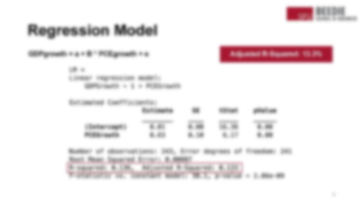
2. Estimate a regression model using one of the variables as a dependent variable and the
other one as an independent variable.
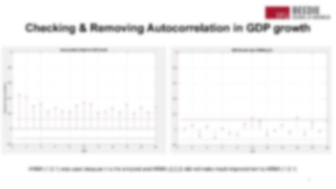
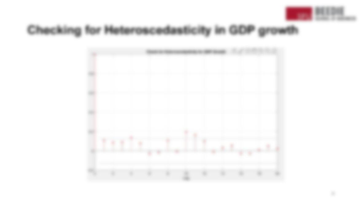
3. Estimate an ARMA/GARCH model for each data series separately to remove any serial
correlation or heteroscedasticity.
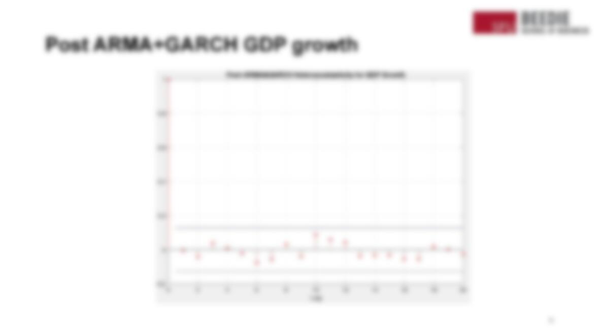
4. Re-estimate the regression from Step 2 above using the standardized residuals from the
ARMA/GARCH models. Compare the results from Step 2 and Step 4.
2
Data Selection
●We used GDP and personal
consumption expenditure as correlation
will exist between them
●There’s evidence that there is mild positive
autocorrelation in the growth of GDP
○It means that if GDP grows faster
than average in one period, there is a
tendency for it to grow faster than
average in the following periods
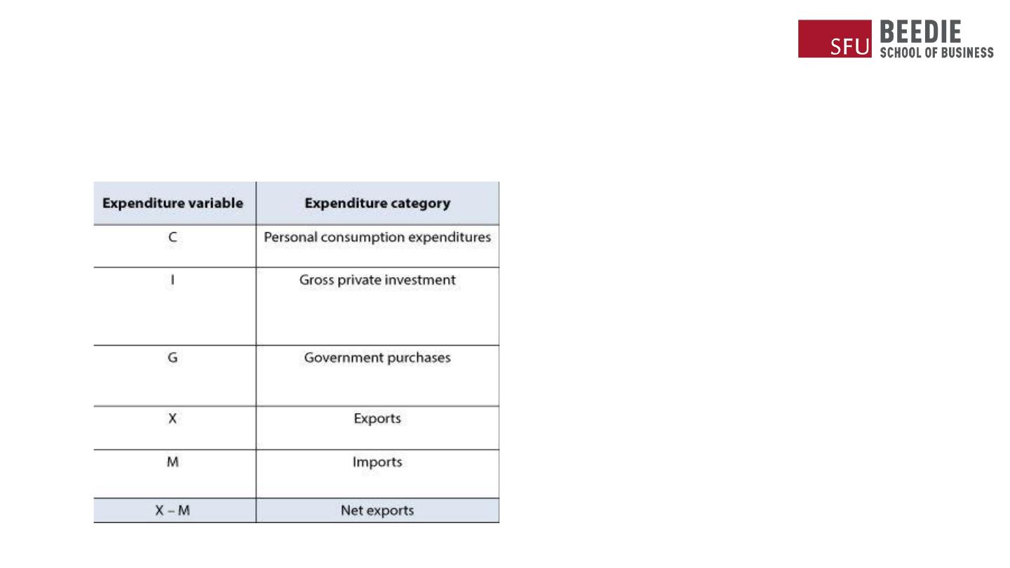
GDP = C + I + G + (X – M)
3
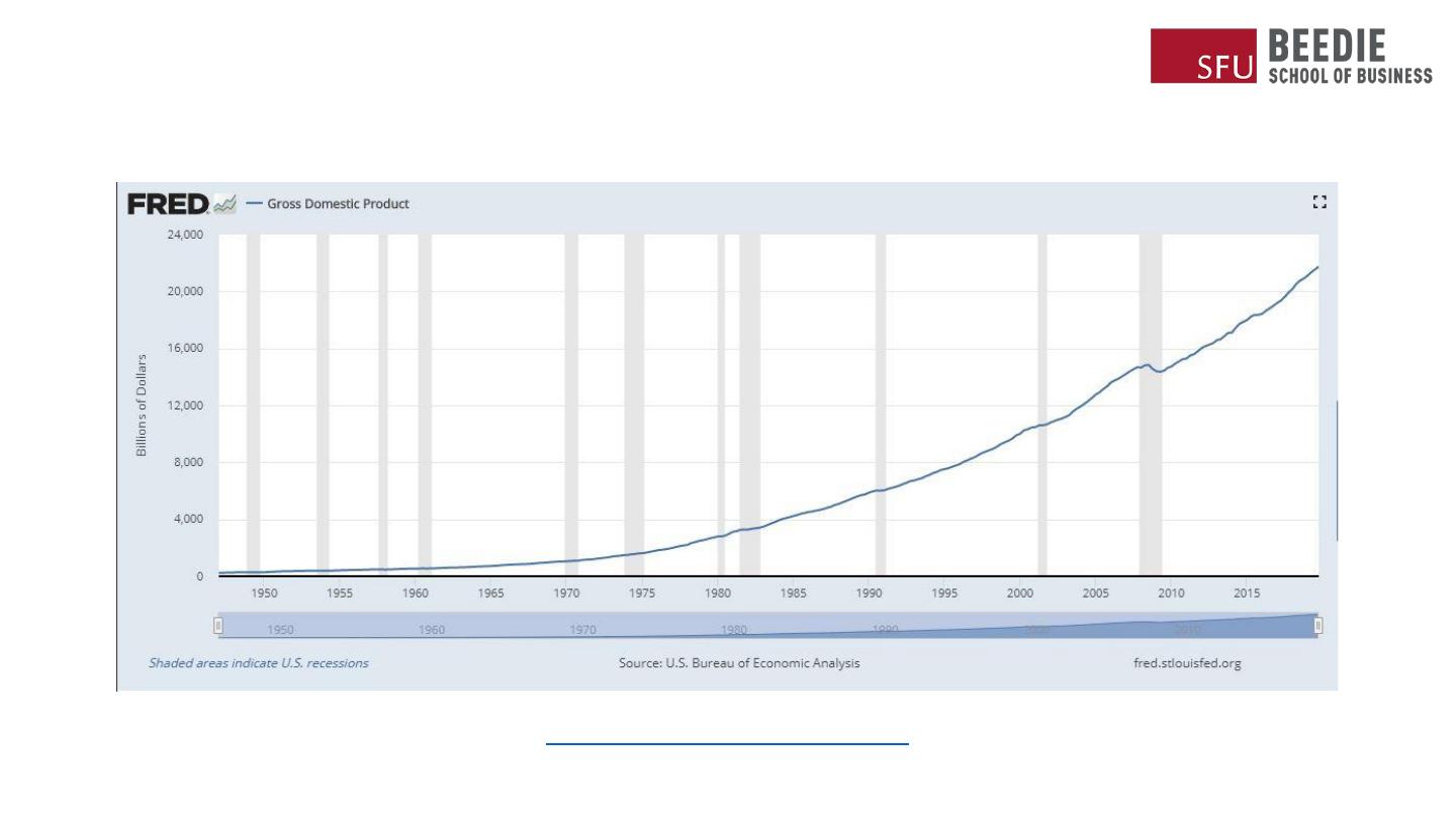
GDP Trend
https://fred.stlouisfed.org/series/GDP
4
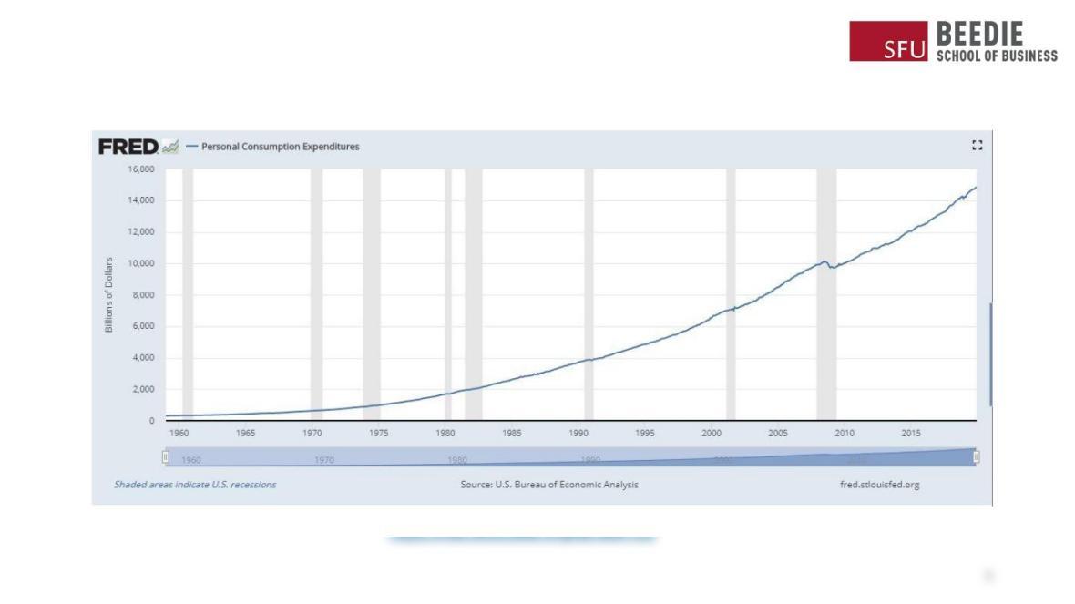
Personal Consumption Expenditure Trend