MBA 646
Professor Carter
Assignment 2 solutions
Ch. 2: 6, 11, 30, Nasdaq
Chapter 2
6. (a)
(b) Because the distribution is reasonably symmetrical, we could use either the mean or median as a
representative value. If the distribution were more strongly skewed to the right, we might prefer the median.
(c) The standard deviation of commuting times is a useful measure of variation = 7.506.
(d) The empirical rule states that for a reasonably symmetrical distribution, approximately 95% of values will
lie within the mean + or – 2 standard deviations. The endpoints are thus 48.093-2*7.506 and 48.093+2*7.093,
i.e. 33.091 and 63.105. After sorting, there are 18 values outside this range so 361 are within which = 95.25%.
This is consistent with the empirical rule.
11.
(a) Appraised Value, Selling Price, and Square Feet are continuous; Bedrooms and Bathrooms are discrete.
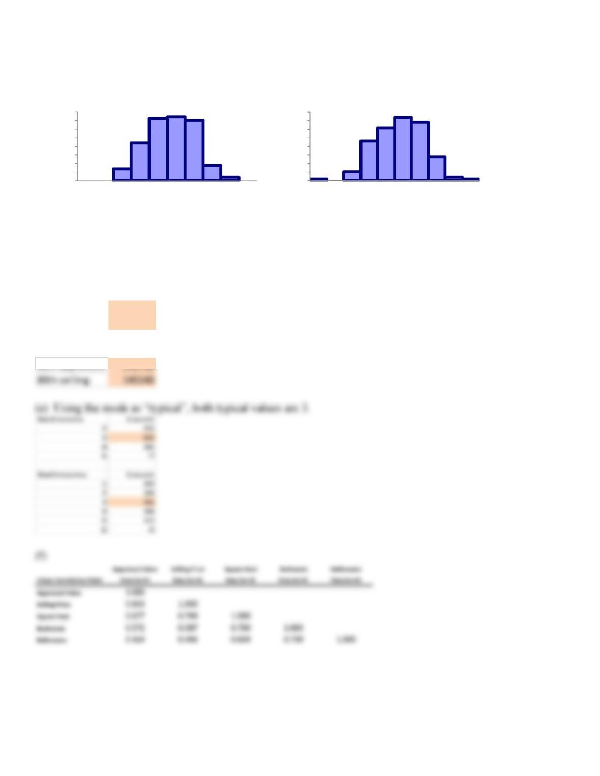
(b) It’s helpful for comparing the distributions to use the same scale and same number of groups for the two
histograms.
0
20
40
60
80
100
120
34.227
38.980
43.733
48.487
53.240
57.993
62.747
67.500
72.253
77.007
Frequency
Average time (mins)
Histogram of Commute Time / Data Set #1
Commute Time
One Variable Summary Data Set #1
Mean 48.093
Std. Dev. 7.506
Median 47.333
Mode 44.017
Minimum 31.850
Maximum 79.383
Count 379
MBA 646
Professor Carter
Assignment 2 solutions
Ch. 2: 6, 11, 30, Nasdaq
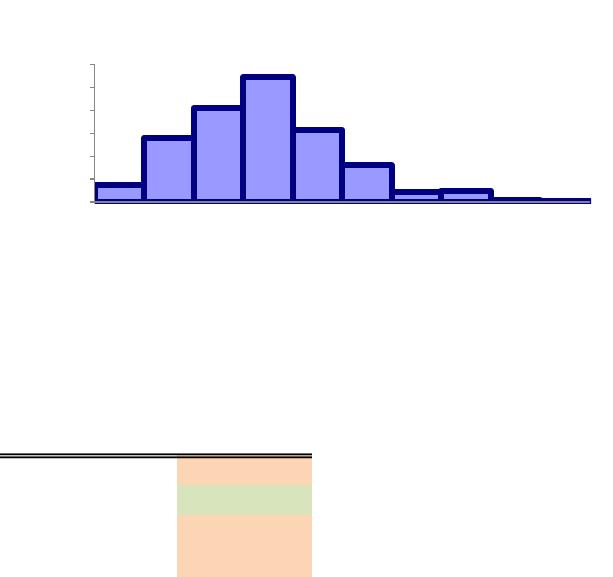
The distributions are both fairly symmetric and bell-shaped, but the selling prices are slightly more spread out.
For each, the “typical” value is around 135000.
(c)
Minimum
1210
Maximum
2510
(d)
0
5
10
15
20
25
30
35
40
85000.00
95000.00
105000.00
115000.00
125000.00
135000.00
145000.00
155000.00
165000.00
175000.00
Frequency
Appraised value
Histogram of Appraised Value / Data Set #1
0
5
10
15
20
25
30
35
40
85000.00
95000.00
105000.00
115000.00
125000.00
135000.00
145000.00
155000.00
165000.00
175000.00
Frequency
Selling price
Histogram of Selling Price / Data Set #1