Applied Economics
Roman Matkovskyy
Roman.Matkovskyy@rennes-sb.com
MARKET STRUCTURES AND
BUSINESS ORGANIZATION

Lecture outline
•Perfect competition
•Profit maximization
•The decision to shut down
•Monopoly
•Profit maximization
•Monopoly power and the Lerner index
•Monopolistic competition –Profit maximization
•Oligopoly/duopoly: quantity competition vs price competition
•the Cournot model
•the Cartel model
•the Stackelberg model
•the Bertrand model
•the Sweezy model

Perfect competition
•A perfectly competitive market is distinguished by the following characteristics:
•A large number of economic players of producers and consumers. They are small enough to
influence the price of product. The price is considered “given” and they are all considered “price
takers.”
•The product is homogeneous across all the producing firms so that consumers would be
indifferent to products of all firms.
•The resources are perfectly mobile, implying that no input of production is monopolized by its
supplier and all firms are free to enter and exit their industry with ease and at no extra cost.
•Economic players are assumed to have perfect knowledge of prices and costs, and market
conditions.
•Economic players incur no extra cost for market transactions or exchanges.
•Although these economic conditions are more of theoretical assumptions than reality, they play
an important role in providing the knowledge to comprehend reality, predict changes, and be able
to exert positive influence and improve it.

Perfect competition
•Do not choose price.
•Choose output quantity. TC includes opportunity cost of capital
invested.
•What will be our profit (loss) from our output decision?
•Should we produce now? (SR)
•Should we stay in the industry? (LR)
Profit Maximization for Competitive Firms
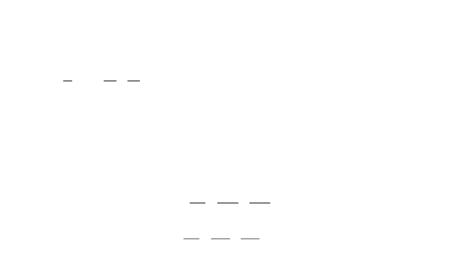
•Profit 𝜋 = 𝑇𝑅 −𝑇𝐶
•FOC: 𝜕𝜋
𝜕𝑄 = 0 → 𝜕𝑇𝑅
𝜕𝑄 −𝜕𝑇𝐶
𝜕𝑄 = 0 → 𝑀𝑅 −𝑀𝐶 = 0 → 𝑀𝑅 =𝑀𝐶
•and this is where the golden rule of the equimarginal principle came from.
•It states that the output would be optimal and the profit would reach its maximum when the
marginal revenue is equal to the marginal cost.
•To prove that this point on the profit curve represents the maximum profit point, we check the second
derivative of the profit.
•If it is found to be negative, point would be the maximum, because then it means that the slope of
the marginal revenue curve is less than the slope of the marginal cost curve:
𝜕2𝜋
𝜕𝑄2=𝜕2𝑇𝑅
𝜕𝑄2−𝜕2𝑇𝐶
𝜕𝑄2
𝜕2𝜋
𝜕𝑄2=𝜕𝑀𝑅
𝜕𝑄 −𝜕𝑀𝐶
𝜕𝑄 0
Profit Maximization for Competitive Firms,
cont
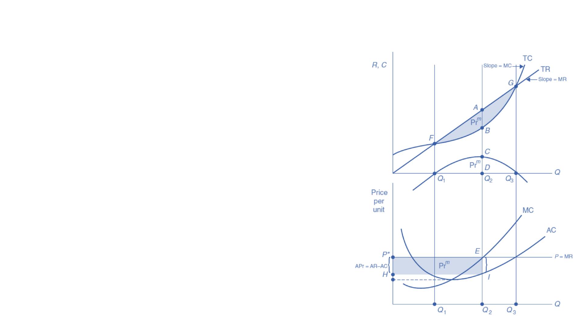
•For a competitive firm, profit maximization in the short run occurs when the
market price of a product is equal to the marginal cost of producing it.
•This is simply because the competitive firm’s demand curve is a horizontal line
determined at the price level and it is equal to the marginal revenue.
•We can observe this on the lower panel of Figure at point E, corresponding to
output level Q2. This point is the point of equilibrium for the competitive firm
where profit is maximized at point C in the upper panel.
•Maximum profit Prmis represented by the longest vertical distance between TR
and TC curves (line AB), which is exactly equal to line CD.
•The shaded area between points F and G is the cumulative profit earned when
producing output level Q1 through Q3. In the lower panel, we can see the total
profit earned by producing the optimum level of output Q2.
•Total profit is represented by the shaded rectangular area where the length is Q2
and the height is the average profit (APr), which is the difference between the
product’s average revenue (AR) and the product’s average cost (AC):
APr = AR − AC,
where the average revenue is essentially the product’s market price:
APr = P − AC.
This is because: APr = 𝑷𝒓/Q= TR/Q –TC/Q. TR = PxQ and TC/Q=AC, APr =
PxQ/Q−TC/Q= P − AC.

Exercise
•A competitive firm has the following cost function:
𝑇𝐶 =20+4𝑄 +0.003𝑄2.
Given that the market price for the firm’s product is $16.00, find the
following:
1. The equilibrium output level that would maximize its profit.
2. How much would be the maximum profit?

Exercise: solution
1. The firm would maximize its profit when its marginal cost is equal to
its marginal revenue.
Being a competitive firm dictates that its marginal revenue is equal to
its product market price ($16.00), we shall find its marginal cost:
𝑀𝐶 =𝜕𝑇𝐶
𝜕𝑄 = 4+0.006𝑄
MC=MR –> 4+0.006𝑄 =16 → 𝑄 = 2000the equilibrium output
level.
2. 𝜋 = TR−TC = P×𝑄 − 20+4𝑄 +0.003𝑄2=16×2000−
20+4×2000+0.003×20002=11980

Exercise
An industry is consisted of 5000 perfectly competitive firms with
market demand and supply function described by
Qd = 35,000 − 20P,
Qs = 5000 + 10P.
1. What would be the profit-maximizing output level for the industry
and what would be the uniform market price for the product?
2. What would be the market share of output for each firm?
3. What would be the marginal cost for each firm?

Exercise
1. Qd = Qs
35,000 − 20P = 5000 + 10P
P=1000
Substituting the market price ($1000) in either the demand or supply equation
would yield the equilibrium quantity of the industry:
Qd = 35,000 − 20×1000=15000
Qs = 5000 + 10×1000=15000
2. Since the industry contains 5000 competitive firms, each firm would produce:
15000/5000=3 units
3. Since the profit-maximizing condition is achieved when P = MR = MC. The
marginal cost should be the same as the price. That is $1000.
The Decision to Shut Down
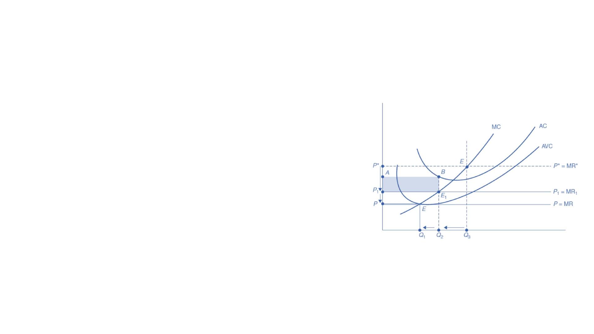
•At the equilibrium price P∗, as shown in Figure, the firm was producing
output level Q2 and earning a total profit equal to the area P∗EIH.
•If the market price falls to a level that would not cover the average cost
such as P1 in the following graph (Figure), which is below the bottom of
the average cost curve (AC), then the equilibrium point would shift to E1
and the company would suffer a loss equal to the area ABE1P1, and the
output would be reduced to Q1. The company would continue to operate
and try to minimize its loss as much as possible.
•However, if the product market price continued to fall further to a level
equal to or below the company’s average variable cost (AVC) such as P,
the firm would rather shut down at this point because the revenue can
no longer cover the fixed cost (FC). So, the decision to shut down is tied
to the fact that the revenue falls below the firm’s short-run variable cost:
•TR VC ->PxQ VC
•Dividing by Q,
•PQ/Q VC/Q –> P AVC (shut-down point)

Exercise
•Consider a competitive firm with a cost function of 𝑇𝐶 =800+
75𝑄 −12𝑄2+2𝑄3.
1. When would this firm prefer to shut down?

Exercise : solution
•Consider a competitive firm with a cost function of 𝑇𝐶 =800+75𝑄 +12𝑄2+2𝑄3.
•1. The firm would shut down when the price of its product falls to a point where the price is equal to its
average variable cost (i.e., P = AVC). So, we have to find the average variable cost:
𝑉𝐶 =75𝑄 −12𝑄2+2𝑄3
𝐴𝑉𝐶 = 75𝑄 −12𝑄2+2𝑄3
𝑄=75−12𝑄 −2𝑄2
•Taking the first derivative of the AVC, setting it to zero, and solving for Q would give us the output level at
which the firm would shut down:
𝜕𝐴𝑉𝐶
𝜕𝑄 = 0 → −12−4𝑄 = 0 → 4𝑄 =12 → 𝑄 = 3
•To find the price, we know that a competitive firm has a price equal to its marginal revenue which is equal to
marginal cost. Marginal cost is the first derivative of the total cost, which is
𝑀𝐶 = 𝜕𝑇𝐶
𝜕𝑄 =75−24𝑄 +6𝑄2
𝑃 = 𝑀𝐶 =75−24𝑄 +6𝑄2=75−24×3+6×32=57
So, the firm would prefer to shut down once the price falls to $57 or below.

Exercise
•Suppose that a competitive firm’s total cost function is
𝑇𝐶 =250+5𝑄 +0.025𝑄2
If the product market price is $15, find the following:
1. What would be the firm’s maximum profit, and at which size of
production?
2. What would be the level of output at which the firm would break
even?
Exercise : solution
1. Let us take the first derivative of the profit function, set it to zero, and
solve it for Q:
π = 𝑃 ×𝑄 − 250+5𝑄 +0.025𝑄2=15𝑄 −250−5𝑄 −0.025𝑄2
=10𝑄 −250−0.025𝑄2
𝜕π
𝜕𝑄 = 0 → 𝜕10𝑄 −250−0.025𝑄2
𝜕𝑄 = 0
10−0.05𝑄 = 0 → 𝑄 = 200units
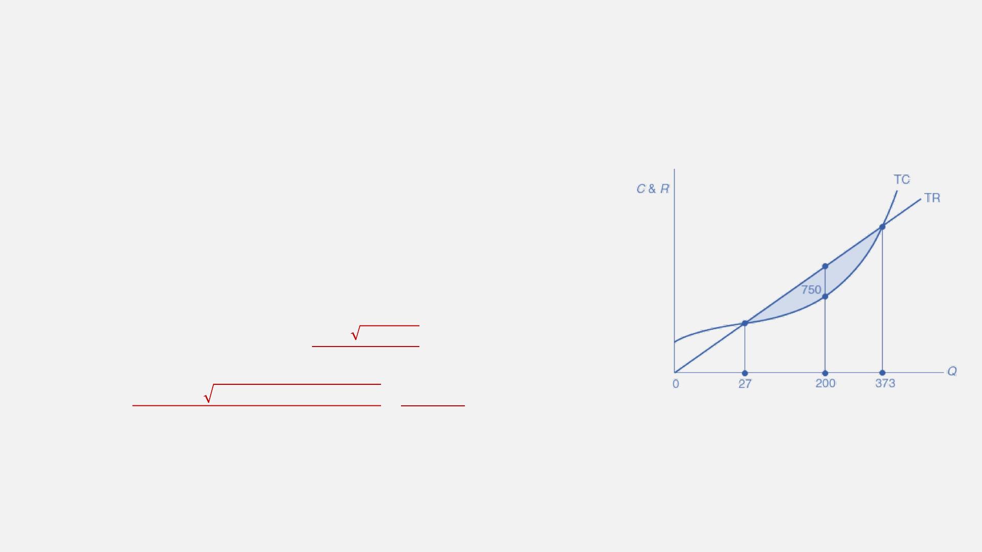
π = 10𝑄 −250−0.025𝑄2=10×200−250−0.025×2002=750
To prove that this is the maximum profit, the second derivative has to be
negative: 𝜕2π
𝜕𝑄2= −0.05 0
Exercise : solution
2. The break-even level of output occurs when the total cost is equal to the total
revenue:
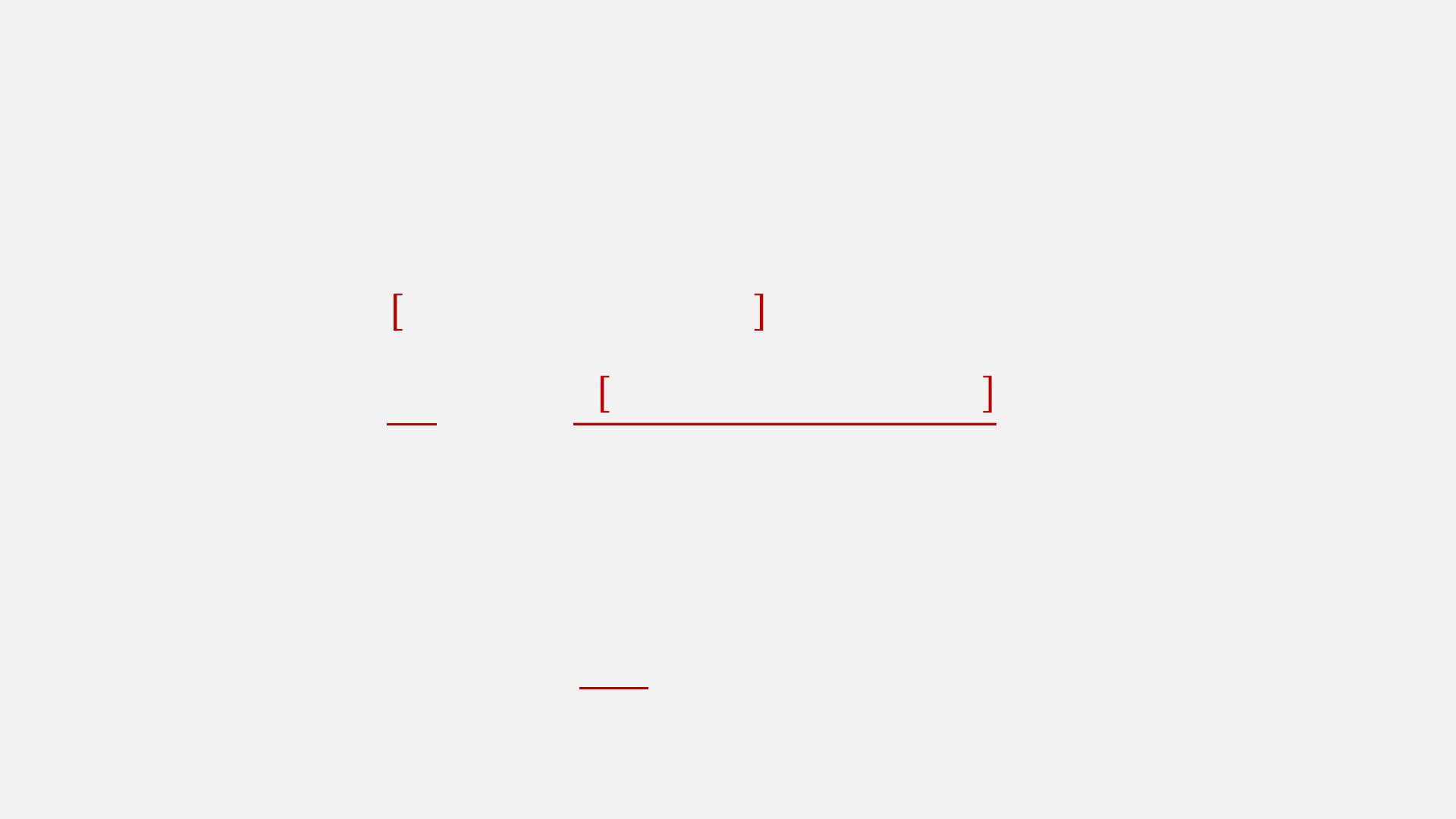
TC=TR 250+5𝑄 +0.025𝑄2=15𝑄
0.025𝑄2−10𝑄 +250 = 0
We use the quadratic formula to solve for Q where
a = 0.025,
b = –10,
c = 250,
𝑄 = −𝑏 ± 𝑏2− 4𝑎𝑐
2𝑎
𝑄 = −(−10)± (−10)2−4×0.025×250
2×0.025 =10±8.66
0.05 ; 𝑄1=373,𝑄2=27
When Q has two values, it means that the firm’s break even is at two different levels of
output, as shown in Figure
Monopoly
At the opposite extreme of perfect competition is the imperfect competition of
the market structure. At the very end of the spectrum of the imperfect
competition is monopoly. It is a market organization that is reverse in terms of
perfect competition. Characteristics of monopoly include the following:
1. A single producer who dominates the production of a unique product, which
has no close substitute.
2. The characteristic mentioned above leads to the natural result that the
monopolistic firm representing the entire industry single handedly has total
control on the market. Although its market power is not unlimited, it is extremely
significant.
3. Based on points 1 and 2 above, the entry of new firms into the industry is
totally blocked, implying that a monopolistic firm can enjoy earning profits in the
long run, unlike its counterparts in the fully competitive industry.
4. Information for the economic agents on production, cost, price, and quality is
not perfect as it is assumed in the perfect competition scenario.
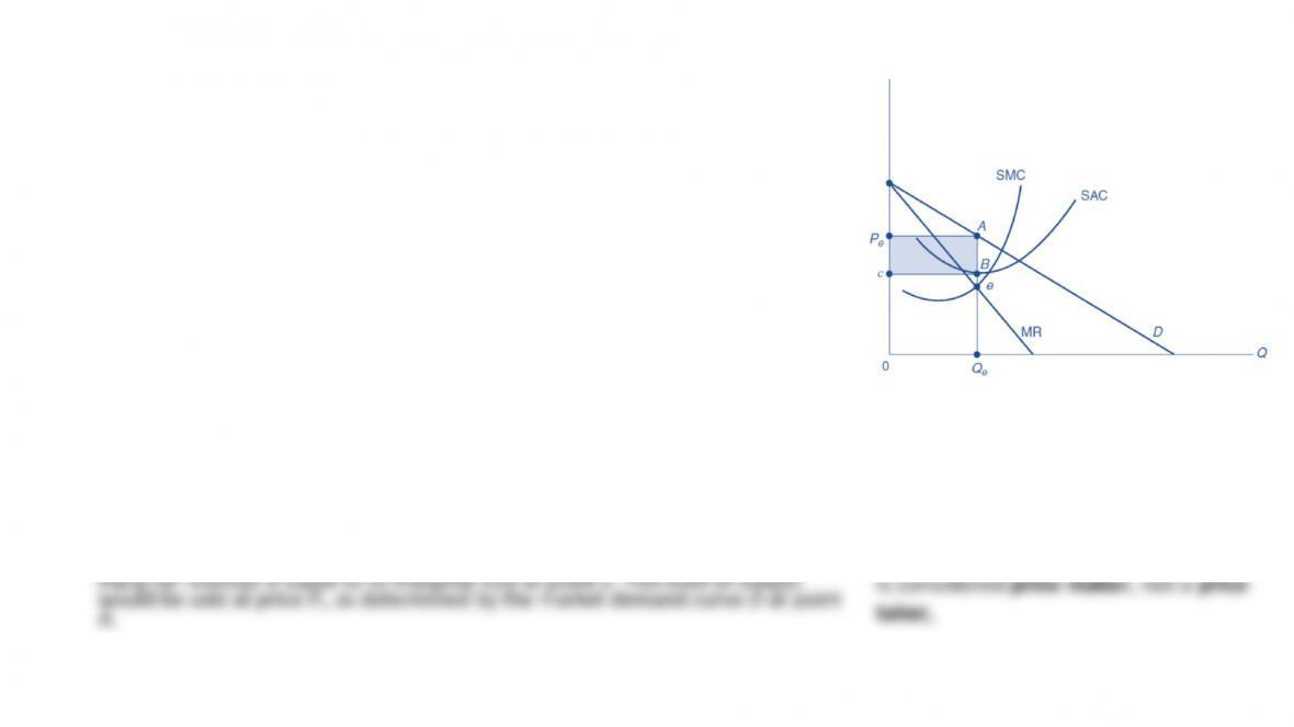
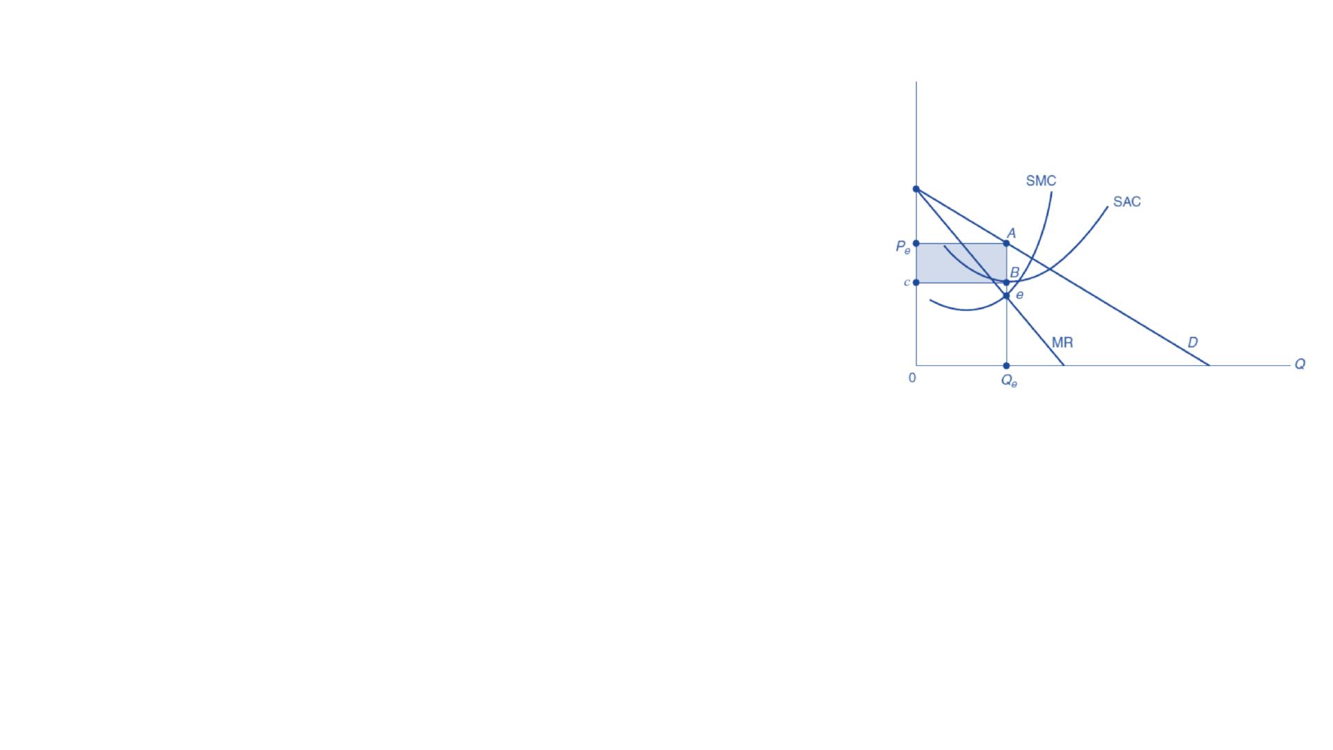
A monopolistic firm would produce its optimum level of output Qe, where its
The price Peis determined indirectly by
the firm because of the firm’s influence
on the quantity, given the state of the
market demand. This is why a monopoly


































B?