Page 1 of 54
ANLY 500 Laboratory #1 – Descriptive
Statistics
Evans Chapter 1 through and including Chapter 7
“Performance Lawn Equipment Case Study” from Evans, Business Analytics
Contents
Introduction ………………………………………………………………………………………………………………………………. 3
Chapter 1 ………………………………………………………………………………………………………………………………….. 5
Step 1 …………………………………………………………………………………………………………………………………… 5
Step 2 …………………………………………………………………………………………………………………………………… 5
Chapter 2 – Optional…………………………………………………………………………………………………………………… 6
Step 1 …………………………………………………………………………………………………………………………………… 6
Step 2 …………………………………………………………………………………………………………………………………… 7
Step 3 …………………………………………………………………………………………………………………………………… 9
Step 4 …………………………………………………………………………………………………………………………………. 11
Chapter 3 ………………………………………………………………………………………………………………………………… 12
Part 1 ………………………………………………………………………………………………………………………………….. 12
Step 1 ……………………………………………………………………………………………………………………………… 12
Step 2 ……………………………………………………………………………………………………………………………… 17
Part 2 ………………………………………………………………………………………………………………………………….. 17
Step 1 ……………………………………………………………………………………………………………………………… 17
Part 3 ………………………………………………………………………………………………………………………………….. 18
Step 1 ……………………………………………………………………………………………………………………………… 18
Step 2 ……………………………………………………………………………………………………………………………… 21
Part 4 ………………………………………………………………………………………………………………………………….. 21
Chapter 4 ………………………………………………………………………………………………………………………………… 21
Part 1 ………………………………………………………………………………………………………………………………….. 21
Step 1 (Part a)…………………………………………………………………………………………………………………… 21
Page 2 of 54
Step 2 (Part b) ………………………………………………………………………………………………………………….. 23
Step 3 (Part c)…………………………………………………………………………………………………………………… 25
Step 4 (Part d) ………………………………………………………………………………………………………………….. 26
Step 5 (Part e)…………………………………………………………………………………………………………………… 27
Chapter 5 ………………………………………………………………………………………………………………………………… 31
Part 1 ………………………………………………………………………………………………………………………………….. 31
Step 1 ……………………………………………………………………………………………………………………………… 31
Step 2 ……………………………………………………………………………………………………………………………… 32
Step 3 ……………………………………………………………………………………………………………………………… 32
Step 4 ……………………………………………………………………………………………………………………………… 33
Step 5 ……………………………………………………………………………………………………………………………… 33
Step 6 ……………………………………………………………………………………………………………………………… 33
Step 7 ……………………………………………………………………………………………………………………………… 34
Step 8 ……………………………………………………………………………………………………………………………… 34
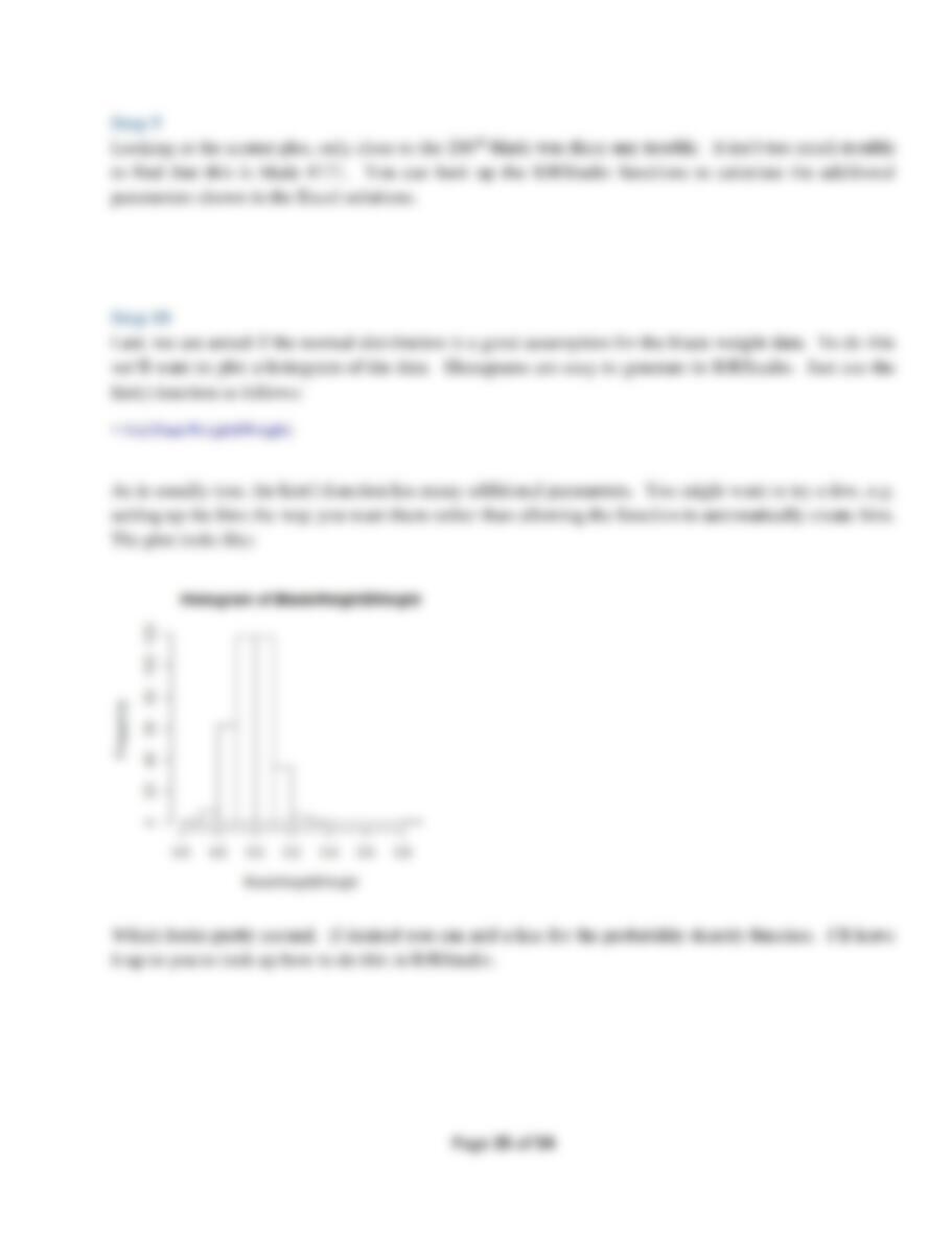
Step 9 ……………………………………………………………………………………………………………………………… 35
Step 10 ……………………………………………………………………………………………………………………………. 35
Chapter 6 ………………………………………………………………………………………………………………………………… 36
Part 1 ………………………………………………………………………………………………………………………………….. 36
Step 1 ……………………………………………………………………………………………………………………………… 36
Step 2 ……………………………………………………………………………………………………………………………… 37
Step 3 ……………………………………………………………………………………………………………………………… 39
Step 4 ……………………………………………………………………………………………………………………………… 39
Step 5 …………………………………………………………………………………………………………………………………. 42
Step 6 …………………………………………………………………………………………………………………………………. 44
Chapter 7 ………………………………………………………………………………………………………………………………. 44
Part 1 …………………………………………………………………………………………………………………………………. 45
Part 2 …………………………………………………………………………………………………………………………………. 46
Part 3 …………………………………………………………………………………………………………………………………. 47
Part 4 …………………………………………………………………………………………………………………………………. 48
Part 5 …………………………………………………………………………………………………………………………………. 49
Summary – Your Laboratory Report ………………………………………………………………………………………….. 51

Page 3 of 54
Introduction
This laboratory follows the exercises in the book, specifically the Performance Lawn Equipment Case
Study homework assigned exercises Chapters 1 through and including 7, except this laboratory requires
that you use R to complete the exercises. That is, you should answer all questions in the textbook
exercises and when necessary to complete computations use R. Each laboratory in ANLY 500 will
build on the laboratories you have completed before. So, you will want to set-up a folder or file to keep
your work in so that you can refer back to previous laboratories if necessary. If you have not used R
before you should install R and RStudio on your computer or laptop. RStudio is a user interface for R
that will make your life and work much easier. To get credit for completing this laboratory you must
submit a report with your results on Moodle.
Once you have installed R and RStudio you may want to browse through some of the packages available
for you. You can do that from the “Quick list of useful R packages” at
https://support.rstudio.com/hc/en-us/articles/201057987-Quick-list-of-useful-R-packages or
https://cran.r-project.org/web/packages/. Essentially what R does is use functions already coded in these
packages to do the computations you want to perform. Each package will have an associated CRAN
package website that provides all the information you need about any package. You can also do a
Boolean search on Google or other browser to find additional information about packages or functions.
If you need a specific package to complete an exercise you will be told which package that is as part of
the exercise.
Unless told you will need to find a data set to use you will be provided data sets through Moodle. This
is true for this laboratory, ANLY 500 Laboratory #1. For this laboratory there are a total of 23 data files
in csv format. There is one data file for each spreadsheet in the Performance Lawn Equipment Excel
Workbook that is also on Moodle. Your first task will be to load these data files into RStudio.
However, before you can begin to read data into RStudio you will need to be able to move around the
folders on your computer.
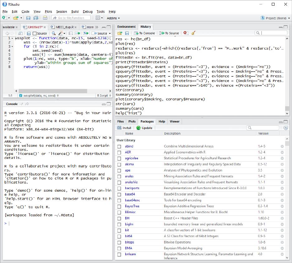
When you start RStudio you will see a number of frames in the RStudio window, going clockwise from
the upper left: a frame showing contents of your R scripts or data objects; an Environment and History
frame; an information frame including your files, plots, packages, help and viewer; and, your Console
frame. This will look something like the figure below:
Page 4 of 54
To find out what folder your default folder is set-up to be you can use the pull down menu “Tools” then
look at your “Global Options”. If you click on “Browse” by the box for your “Default working
directory” it will take you to the directory that RStudio goes to automatically when you start RStudio. If
you want to change this directory just browse to the one you want to use and accept that change. I
strongly suggest you set-up a separate directory just for your R/RStudio work. I have one I names
“MyRWork” and within that folder I have a “data” folder and other folders for specific projects, etc.
The function to find out what directory you are actually in is getwd() which simply stands for get
working directory. That is the syntax you need to use. The parentheses, which are empty, return the
current directory. To change directory the function is setwd(). So, for example if I am in my default
working directory “MyRWork” and want to go to my data directory I enter setwd(“data”) in the console
frame. The quotation marks are necessary. R distinguishes between names with no quotation marks,
single or double quotation marks and treats each entry differently. So, for the directory name use the

Page 5 of 54
double quotation marks around it. If things are not working quite right, e.g. RStudio isn’t reading files,
chances are you are not in the correct directory.
Once you are in the directory where you’ve downloaded the data files you can load the data into
RStudio. You can do this automatically using the pull down menu “Tools” then “Import Dataset”.
Doing this you choose a “From Local File” or “From Web URL”. Since these will be on your computer
or laptop choose “From Local File” then just go to the appropriate directory and select the data file you
want to import. Or you can immediate begin using R’s functions for reading in data using the following
command in the Console frame:
> BladeWeight <- read.csv(“~/MyRWork/data/Evans/BladeWeight.csv”)
You have extensive help files available through RStudio. To get help, in the Console use the help()
function and the function name you need help with in double quotations, e.g.
> help(“read.csv“)
One thing to watch out for, whether you use the pull down menu to import or the command line, is that
the column headings are recognized. For some reason when I read or import the Evans’ data files some
files recognize headings and other do not. So, be careful about this.
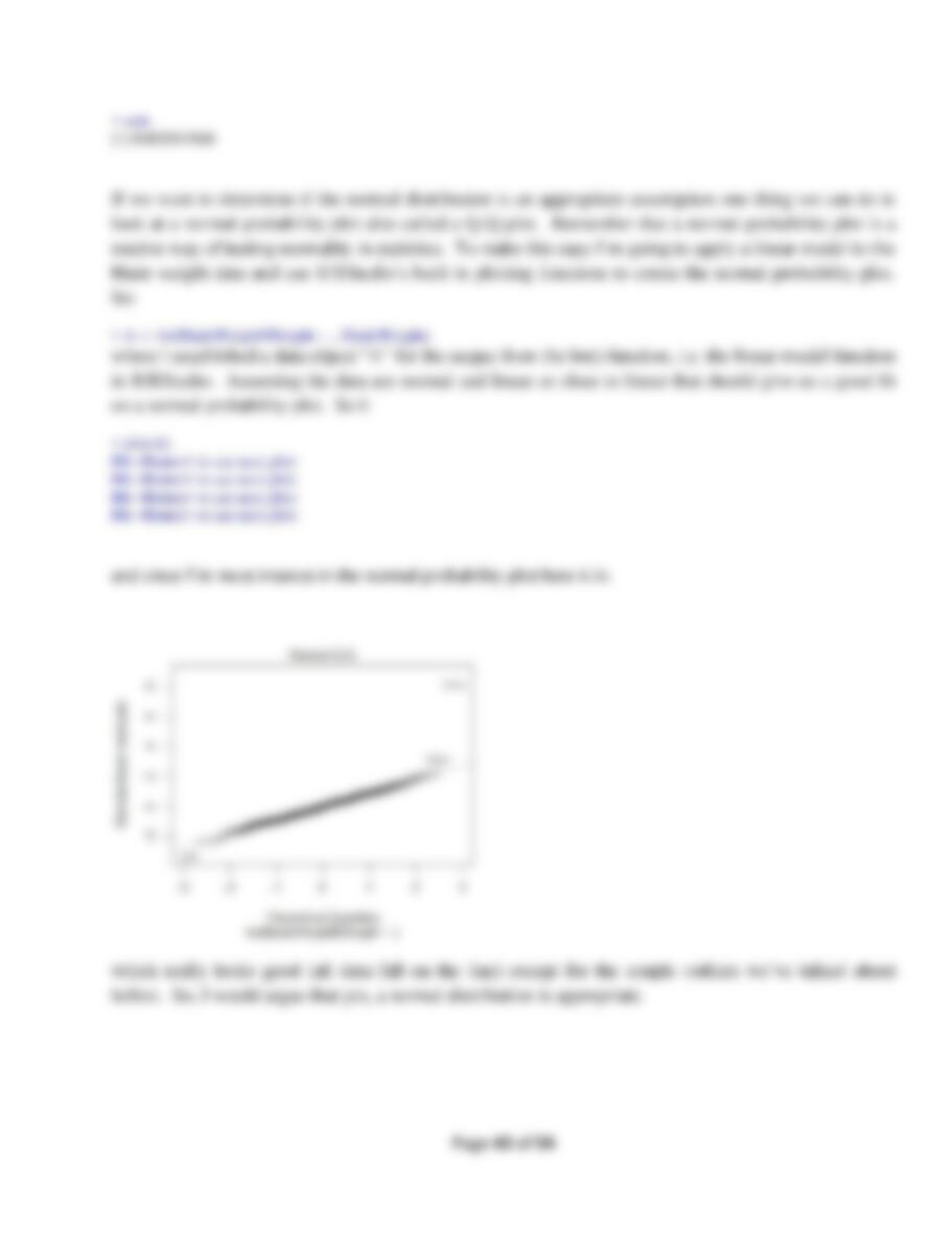
Chapter 1
Step 1
Read the data files for Performance Lawn Equipment (PLE) into R/RStudio.
Step 2
Determine the data type for each variable in the PLE data files.
It is easy to determine the data types for variables in R. Simply use the str() function with the data
filename or data object in the parentheses. For example,
> str(BladeWeight)
‘data.frame’: 350 obs. of 2 variables:
$ Sample: int 1 2 3 4 5 6 7 8 9 10 …
$ Weight: num 4.88 4.92 5.02 4.97 5 4.99 4.86 5.07 5.04 4.87 ...

Page 6 of 54
For the BladeWeight data file the str() function returns the information that there are 350 observations of
2 variables, sample and weight. The sample variable is an integer variable. The weight variable is a
numeric variable. You can use the str() function for each data file to determine the data type of all
variables. Let’s consider one more of the data files in detail, i.e. the EmployeeRetention data file.
Using the str() function we get:
> str(EmployeeRetention)
‘data.frame’: 40 obs. of 7 variables:
$ YearsPLE : num 10 10 10 10 9.6 8.5 8.4 8.4 8.2 7.9 …
$ YrsEducation: int 18 16 18 18 16 16 17 16 18 15 ...
$ College.GPA : num 3.01 2.78 3.15 3.86 2.58 2.96 3.56 2.64 3.43 2.75 …
$ Age : int 33 25 26 24 25 23 35 23 32 34 …
$ Gender : Factor w/ 2 levels “F”,”M“: 1 2 2 1 1 2 2 2 1 2 …
$ College.Grad: Factor w/ 2 levels “N”,”Y”: 2 2 2 2 2 2 2 2 2 1 …
$ Local : Factor w/ 2 levels “N”,”Y”: 2 2 1 2 2 2 2 2 2 2 …
where we have 40 observations for the 7 listed variables. Gender, College Grad, and Local are all listed
as “Factor” variables. This is the same as a categorical variable. If you are not familiar with different
data types you should take some time to look into this. One source you can use is:
https://www.tutorialspoint.com/r/r_data_types.htm.
Chapter 2 – Optional
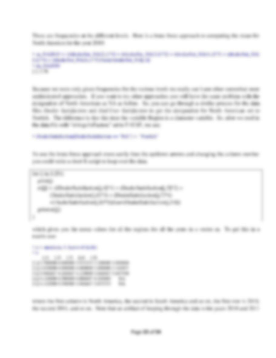
Step 1
Find the total number of responses to each level of the surveys, Dealer and End-User Satisfaction, across
all regions for each year.
To do this we’ll need to subset the data by level and by year. Subsetting data is a standard part of data
analysis. As you will find with most things in R there are many ways of doing this. You can find lots of
information about this online. For example, because the data is essentially in the format of a matrix you
could use row and column numbers – if you know those. You can also use variable names or values.
For example,
> y2010 <- DealerSatisfaction[ which(DealerSatisfaction$Year == 2010), ]
establishes a new data object “y2010” and redirects observations from the DealerSatisfaction data file
into it in which the Year equals 2010. We can see the contents of “y2010” be just typing it on the
command line in the Console.
> y2010
Region Year L0 L1 L2 L3 L4 L5 Count

Page 7 of 54
1 <NA> 2010 1 0 2 14 22 11 50
6 SA 2010 0 0 0 2 6 2 10
11 EU 2010 0 0 1 3 7 4 15
16 PA 2010 0 0 1 2 2 0 5
Things to note include the syntax for the data filename and variable separated by a $, e.g.
DealerSatisfaction and Year as DealerSatisfaction$Year. To designate the test for “equals” use a double
==. You can use this syntax to find all the data required for this step. One of the really nice things
about RStudio is that you can move between commands you have used by the “up” and “down” arrows
on your keyboard. So, to go to the next year you only need to use the up arrow twice to go to the
command to subset the data and then change the year to 2011 to get the answers for the next year, and so
on. When you get to the part that asks for this data for End-User Satisfaction you just need to use the up
arrow appropriately and change the file name.
DO NOT forget to change the data object name for each command you use to store your results in. If
you do not change the data object name you will be continuously writing over your previous results.
To find the sum by year and return the value use the information you got before and sum, e.g.:
> y2010L0 <- sum(y2010[,3])
> y2010L0
[1] 1
That is, the sum for the year 2010 for all regions is 1. You can do this for all the instances you need to.
Choose data object names that make sense so that as you need them you can easily find them again and
again.
Keep in mind that R uses typical matrix notation, i.e. [rows, columns]. So you can always find the value
in an element in a matrix by its [row, column] designation.
Step 2
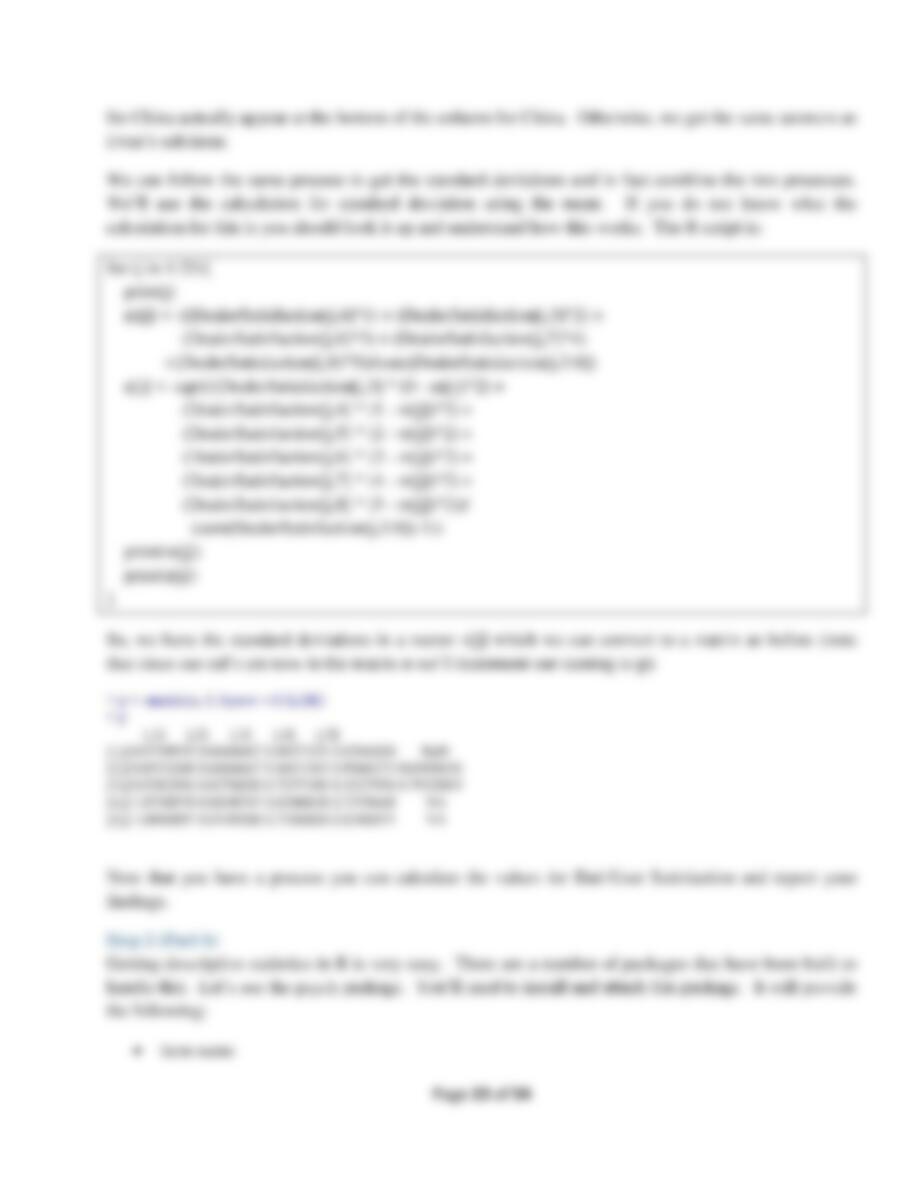
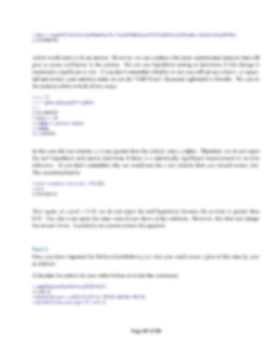
Find the number of failures in the Mower Test.
When the author completed this in Excel he just used the “COUNTIF” function for each column of his
spreadsheet Mower Test. This will take a bit more syntax in R but is relatively easy using the sapply()
function. There is actually a whole family of “apply” functions; e.g. apply, sapply, lapply, etc. All are
helpful in their way so check them out, e.g. in the answer at
http://stackoverflow.com/questions/3505701/r-grouping-functions-sapply-vs-lapply-vs-apply-vs-tapply-
vs-by-vs-aggrega. For our question, we’ll use sapply() and the data file MowerTest but exclude the first
column which is the variable “Observations”. We’ll return the values of “Pass” and “Fail” as a table for
each of the Samples 1 through 30. The syntax we’ll use is:

Page 8 of 54
> y <- t(sapply(MowerTest[-1], function(x) table(factor(x, levels = c(“Pass”, “Fail”)))))
for which y returns:
> y
Pass Fail
Sample.1 97 3
Sample.2 96 4
Sample.3 99 1
Sample.4 100 0
Sample.5 99 1
Sample.6 95 5
Sample.7 98 2
Sample.8 99 1
Sample.9 100 0
Sample.10 98 2
Sample.11 98 2
Sample.12 97 3
Sample.13 97 3
Sample.14 99 1
Sample.15 99 1
Sample.16 98 2
Sample.17 98 2
Sample.18 97 3
Sample.19 98 2
Sample.20 96 4
Sample.21 98 2
Sample.22 99 1
Sample.23 99 1
Sample.24 98 2
Sample.25 99 1
Sample.26 100 0
Sample.27 98 2
Sample.28 99 1
Sample.29 100 0
Sample.30 98 2
You’ll find these are the same totals as Evans shows in his solution. Unfortunately, sapply() has not
returned this as a data.frame from which we could simply find the total number of “Fail”. So, we’ll
convert the output of sapply() into a data.frame and show the output as:
> y2 <- as.data.frame(y)
> str(y2)
‘data.frame’: 30 obs. of 2 variables:
$ Pass: int 97 96 99 100 99 95 98 99 100 98 …
$ Fail: int 3 4 1 0 1 5 2 1 0 2 …

Page 9 of 54
Since y2 is a data.frame we can just use the sum() function to get the total number of “Fail” as follows:
> sum(y2$Fail)
[1] 54
which again matches Evans solutions.
Step 3
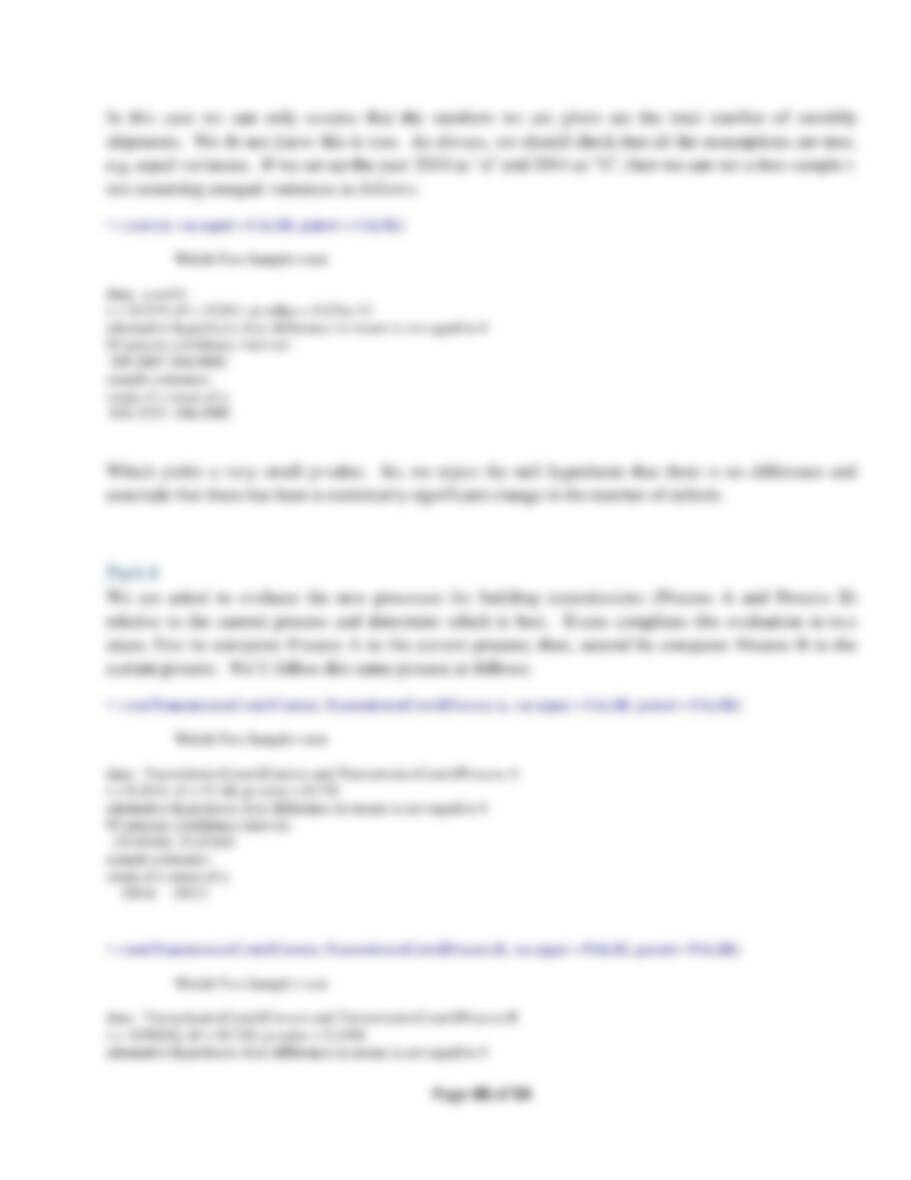
Compute the gross revenue by months and region as well as worldwide for each product using the data
in Mower Unit Sales and Tractor Unit Sales.
We have the numbers of units sold and the price per unit so we just need to compute the gross revenue.
I haven’t really stressed it yet but, as always, the first thing to do is look at the data, use the str() and
summary() functions as follows:
> str(MowerUnitSales)
‘data.frame’: 60 obs. of 8 variables:
$ Month : Factor w/ 12 levels “April”,”August”,..: 5 4 8 1 9 7 6 2 12 11 …
$ Year : int 2010 2010 2010 2010 2010 2010 2010 2010 2010 2010 …
$ NA. : int 6000 7950 8100 9050 9900 10200 8730 8140 6480 5990 …
$ SA : int 200 220 250 280 310 300 280 250 230 220 …
$ Europe : int 720 990 1320 1650 1590 1620 1590 1560 1590 1320 …
$ Pacific: int 100 120 110 120 130 120 140 130 130 120 …
$ China : int 0 0 0 0 0 0 0 0 0 0 …
$ World : int 7020 9280 9780 11100 11930 12240 10740 10080 8430 7650 …
> summary(MowerUnitSales)
Month Year NA.
April : 5 Min. :2010 Min. : 4350
August : 5 1st Qu.:2011 1st Qu.: 5998
December: 5 Median :2012 Median : 7870
February: 5 Mean :2012 Mean : 7542
January : 5 3rd Qu.:2013 3rd Qu.: 9050
July : 5 Max. :2014 Max. :10370
(Other) :30
SA Europe Pacific
Min. :180.0 Min. : 300 Min. :100.0
1st Qu.:250.0 1st Qu.: 840 1st Qu.:140.0
Median :280.0 Median :1260 Median :170.0
Mean :282.3 Mean :1149 Mean :172.5
3rd Qu.:310.0 3rd Qu.:1440 3rd Qu.:202.5
Max. :390.0 Max. :1650 Max. :240.0
China World
Min. : 0.000 Min. : 5350
1st Qu.: 0.000 1st Qu.: 7335
Median : 0.000 Median : 9390

Page 10 of 54
Mean : 1.883 Mean : 9148
3rd Qu.: 0.000 3rd Qu.:10999
Max. :26.000 Max. :12280
> str(TractorUnitSales)
‘data.frame’: 60 obs. of 8 variables:
$ Month: Factor w/ 12 levels “April”,”August”,..: 5 4 8 1 9 7 6 2 12 11 …
$ Year : int 2010 2010 2010 2010 2010 2010 2010 2010 2010 2010 …
$ NA. : int 570 611 630 684 650 600 512 500 478 455 …
$ SA : int 250 270 260 270 280 270 264 280 290 280 …
$ Eur : int 560 600 680 650 580 590 760 645 650 670 …
$ Pac : int 212 230 240 263 269 280 290 270 263 258 …
$ China: int 0 0 0 0 0 0 0 0 0 0 …
$ World: int 1592 1711 1810 1867 1779 1740 1826 1695 1681 1663 …
> summary(TractorUnitSales)
Month Year NA.
April : 5 Min. :2010 Min. : 360.0
August : 5 1st Qu.:2011 1st Qu.: 637.5
December: 5 Median :2012 Median : 835.0
February: 5 Mean :2012 Mean :1075.0
January : 5 3rd Qu.:2013 3rd Qu.:1407.5
July : 5 Max. :2014 Max. :2490.0
(Other) :30
SA Eur Pac
Min. : 250.0 Min. :480.0 Min. :190.0
1st Qu.: 412.5 1st Qu.:577.5 1st Qu.:250.0
Median : 605.0 Median :647.5 Median :270.0
Mean : 598.4 Mean :648.0 Mean :272.2
3rd Qu.: 806.2 3rd Qu.:720.0 3rd Qu.:300.0
Max. :1002.0 Max. :888.0 Max. :350.0
China World
Min. : 0.00 Min. :1592
1st Qu.: 0.00 1st Qu.:1962
Median : 23.00 Median :2408
Mean : 46.65 Mean :2640
3rd Qu.:100.50 3rd Qu.:3222
Max. :139.00 Max. :4476
> str(Prices)
‘data.frame’: 5 obs. of 3 variables:
$ Year : int 2010 2011 2012 2013 2014
$ Mower.Price : int 150 175 180 185 190
$ Tractor.Price: int 3250 3400 3600 3700 3800
> summary(Prices)
Year Mower.Price Tractor.Price
Min. :2010 Min. :150 Min. :3250
1st Qu.:2011 1st Qu.:175 1st Qu.:3400
Median :2012 Median :180 Median :3600
Mean :2012 Mean :176 Mean :3550
3rd Qu.:2013 3rd Qu.:185 3rd Qu.:3700

Page 11 of 54
Max. :2014 Max. :190 Max. :3800
We have prices by year for mowers and tractors. So, we’ll need to subset our mower and tractor data
and apply the correct price by year. There are some things we know that we can use to do this, e.g. each
year has 12 months. So we can subset our data in sets of 12 observations (12 months) and multiply the
number of units by the appropriate price. We know that the first two columns are the month and year
and will have to be omitted from the computations. One way to do this is to subset the data by rows and
columns to get:
> mowerRev2010 <- MowerUnitSales[1:12, 3:8] * Prices[1,2]
> mowerRev2010
NA. SA Europe Pacific China World
1 900000 30000 108000 15000 0 1053000
2 1192500 33000 148500 18000 0 1392000
3 1215000 37500 198000 16500 0 1467000
4 1357500 42000 247500 18000 0 1665000
5 1485000 46500 238500 19500 0 1789500
6 1530000 45000 243000 18000 0 1836000
7 1309500 42000 238500 21000 0 1611000
8 1221000 37500 234000 19500 0 1512000
9 972000 34500 238500 19500 0 1264500
10 898500 33000 198000 18000 0 1147500
11 798000 31500 148500 19500 0 997500
12 696000 27000 99000 21000 0 843000
You can do this for all the years for both mowers and tractors. Or, you can use the more complicated
syntax of one of the “apply()” functions.
Step 4
Now that you have the revenue for mower and tractor sales you can easily find the market share. In fact,
I would have done this by year but in Evans solutions he only shows the answer by region for all five
years combined. You simply find the total gross mower revenue by region, the sum() function properly
applied will do that, and then divide that by the Industry data. You follow the same procedure for the
market share of tractor sales. Be sure to provide your results and summary of results in your laboratory
report.
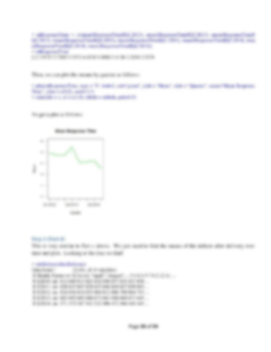
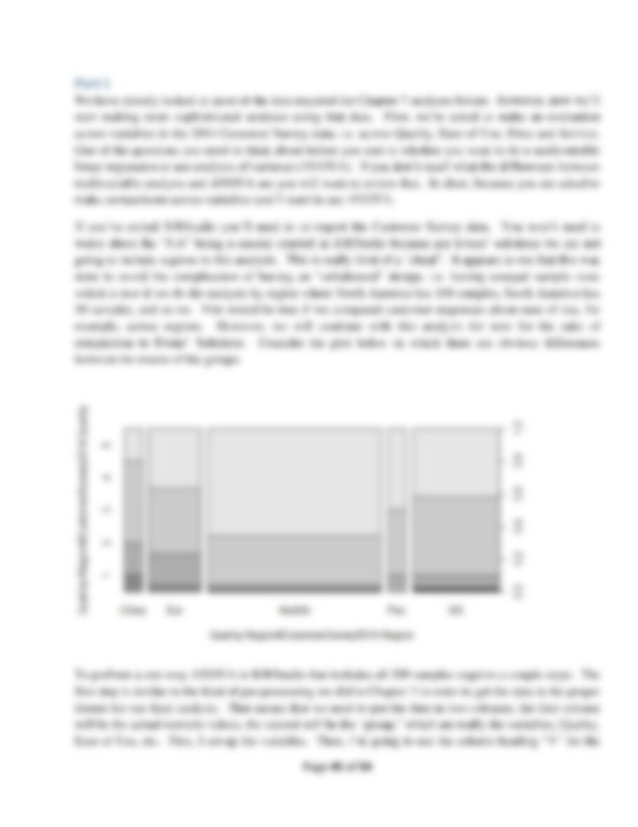
Chapter 3
Part 1
You have been tasked with putting together an overview of PLE’s business performance and market
position. You have specifically been asked to construct appropriate charts and summarize your
conclusions for:
a. Dealer Satisfaction
b. End-User Satisfaction
c. Complaints
d. Mower Unit Sales
e. Tractor Unit Sales
f. On-Time Delivery
g. Defects after Delivery
h. Response Time
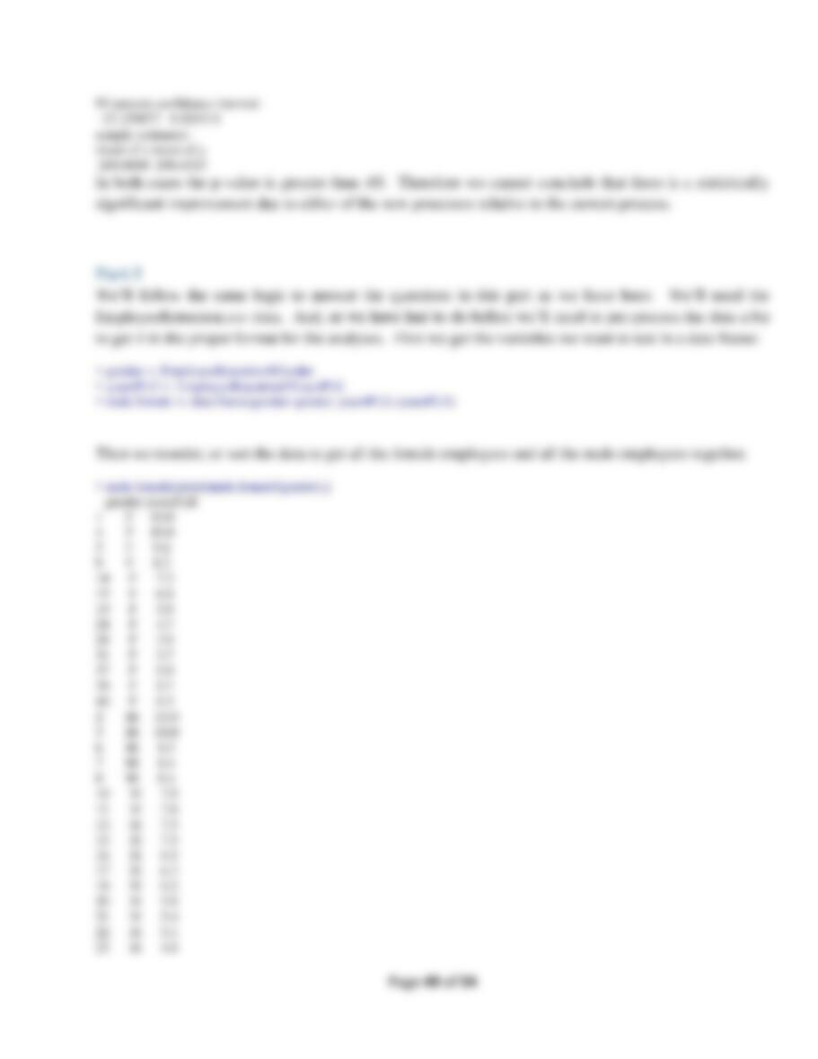
Step 1
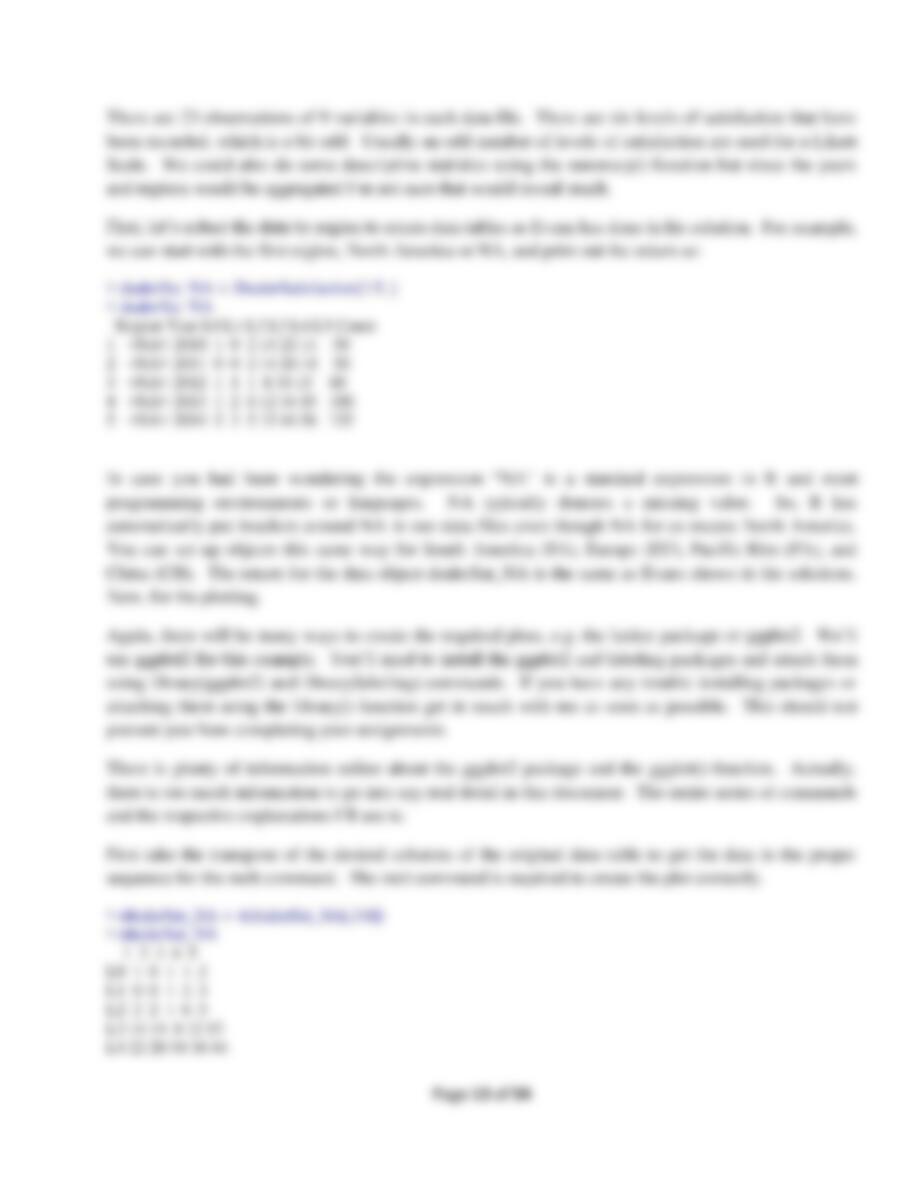
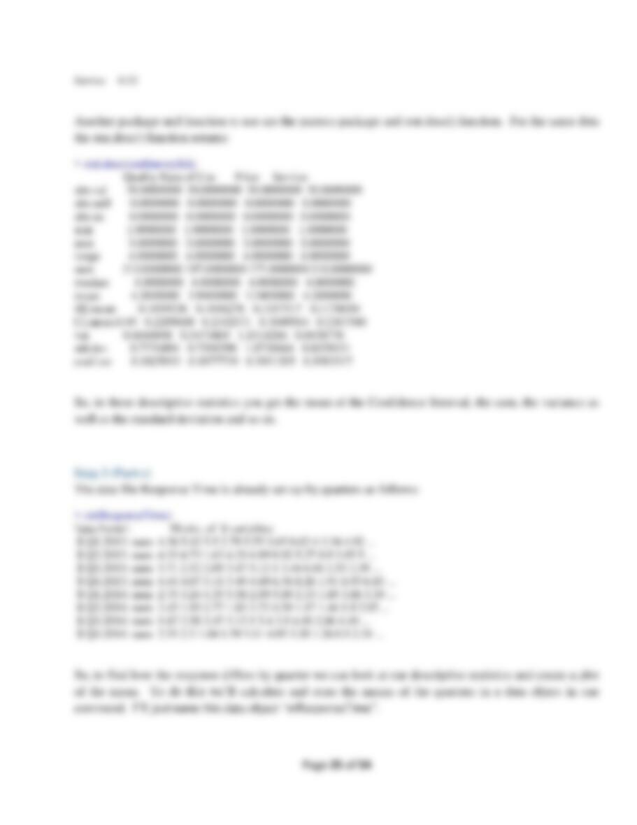
To begin this we’ll again need to put together subsets of the data, e.g. Dealer Satisfaction for North
America, and so on. Once we are through subsetting the data we can create the plots that describe what
is going on performance wise. But first, let’s look at the data:
> str(DealerSatisfaction)
‘data.frame’: 23 obs. of 9 variables:
$ Region: Factor w/ 4 levels “CH”,”EU”,“PA”,..: NA NA NA NA NA 4 4 4 4 4 …