Page 1 of 48
ANLY 500 Laboratory #1 – Descriptive Statistics
1. File Needed: Performance Lawn Equipment Database excel file
2. You will need to select required sheets from the above excel file, convert it
into CSV file and clean it (e.g. remove headers) before using with R.
3. Lab Report # 1 is due 08/19
Evans Chapter 1 through and including Chapter 7
“Performance Lawn Equipment Case Study” from Evans, Business Analytics
Contents
Introduction ………………………………………………………………………………………………………………………………. 1
Chapter 1 ………………………………………………………………………………………………………………………………….. 4
Chapter 2 – Optional…………………………………………………………………………………………………………………… 5
Chapter 3 ………………………………………………………………………………………………………………………………… 10
Chapter 4 ………………………………………………………………………………………………………………………………… 20
Chapter 5 ………………………………………………………………………………………………………………………………… 30
Chapter 6 ………………………………………………………………………………………………………………………………… 35
Chapter 7 ………………………………………………………………………………………………………………………………. 43
Summary – Your Laboratory Report ………………………………………………………………………………………….. 44
Sample report Chapter 1: ………………………………………………………………………………………………………….. 47
Introduction
This laboratory follows the exercises in the book, specifically the Performance Lawn Equipment Case
Study homework assigned exercises Chapters 1 through and including 7, except this laboratory requires
that you use R to complete the exercises. That is, you should answer all questions in the textbook
exercises and when necessary to complete computations use R. Each laboratory in ANLY 500 will
build on the laboratories you have completed before. So, you will want to set-up a folder or file to keep
your work in so that you can refer back to previous laboratories if necessary. If you have not used R
before you should install R and RStudio on your computer or laptop. RStudio is a user interface for R

Page 2 of 48
that will make your life and work much easier. To get credit for completing this laboratory you must
submit a report with your results on Moodle.
Once you have installed R and RStudio you may want to browse through some of the packages available
for you. You can do that from the “Quick list of useful R packages” at
https://support.rstudio.com/hc/en-us/articles/201057987-Quick-list-of-useful-R-packages or
https://cran.r-project.org/web/packages/. Essentially what R does is use functions already coded in these
packages to do the computations you want to perform. Each package will have an associated CRAN
package website that provides all the information you need about any package. You can also do a
Boolean search on Google or other browser to find additional information about packages or functions.
If you need a specific package to complete an exercise you will be told which package that is as part of
the exercise.
Unless told you will need to find a data set to use you will be provided data sets through Moodle. This
is true for this laboratory, ANLY 500 Laboratory #1. For this laboratory there are a total of 23 data files
in csv format. There is one data file for each spreadsheet in the Performance Lawn Equipment Excel
Workbook that is also on Moodle. Your first task will be to load these data files into RStudio.
However, before you can begin to read data into RStudio you will need to be able to move around the
folders on your computer.
When you start RStudio you will see a number of frames in the RStudio window, going clockwise from
the upper left: a frame showing contents of your R scripts or data objects; an Environment and History
frame; an information frame including your files, plots, packages, help and viewer; and, your Console
frame. This will look something like the figure below:
Page 3 of 48
To find out what folder your default folder is set-up to be you can use the pull down menu “Tools” then
look at your “Global Options”. If you click on “Browse” by the box for your “Default working
directory” it will take you to the directory that RStudio goes to automatically when you start RStudio. If
you want to change this directory just browse to the one you want to use and accept that change. I
strongly suggest you set-up a separate directory just for your R/RStudio work. I have one I names
“MyRWork” and within that folder I have a “data” folder and other folders for specific projects, etc.
The function to find out what directory you are actually in is getwd() which simply stands for get
working directory. That is the syntax you need to use. The parentheses, which are empty, return the
current directory. To change directory the function is setwd(). So, for example if I am in my default
working directory “MyRWork” and want to go to my data directory I enter setwd(“data”) in the console
frame. The quotation marks are necessary. R distinguishes between names with no quotation marks,
single or double quotation marks and treats each entry differently. So, for the directory name use the

Page 4 of 48
double quotation marks around it. If things are not working quite right, e.g. RStudio isn’t reading files,
chances are you are not in the correct directory.
Once you are in the directory where you’ve downloaded the data files you can load the data into
RStudio. You can do this automatically using the pull down menu “Tools” then “Import Dataset”.
Doing this you choose a “From Local File” or “From Web URL”. Since these will be on your computer
or laptop choose “From Local File” then just go to the appropriate directory and select the data file you
want to import. Or you can immediate begin using R’s functions for reading in data using the following
command in the Console frame:
> BladeWeight <- read.csv(“~/MyRWork/data/Evans/BladeWeight.csv”)
You have extensive help files available through RStudio. To get help, in the Console use the help()
function and the function name you need help with in double quotations, e.g.
> help(“read.csv”)
One thing to watch out for, whether you use the pull down menu to import or the command line, is that
the column headings are recognized. For some reason when I read or import the Evans’ data files some
files recognize headings and other do not. So, be careful about this.
Chapter 1
Step 1
Read the data files for Performance Lawn Equipment (PLE) into R/RStudio.
Step 2
Determine the data type for each variable in the PLE data files.
It is easy to determine the data types for variables in R. Simply use the str() function with the data
filename or data object in the parentheses. For example,
> str(BladeWeight)
‘data.frame’: 350 obs. of 2 variables:
$ Sample: int 1 2 3 4 5 6 7 8 9 10 …
$ Weight: num 4.88 4.92 5.02 4.97 5 4.99 4.86 5.07 5.04 4.87 …

Page 5 of 48
For the BladeWeight data file the str() function returns the information that there are 350 observations of
2 variables, sample and weight. The sample variable is an integer variable. The weight variable is a
numeric variable. You can use the str() function for each data file to determine the data type of all
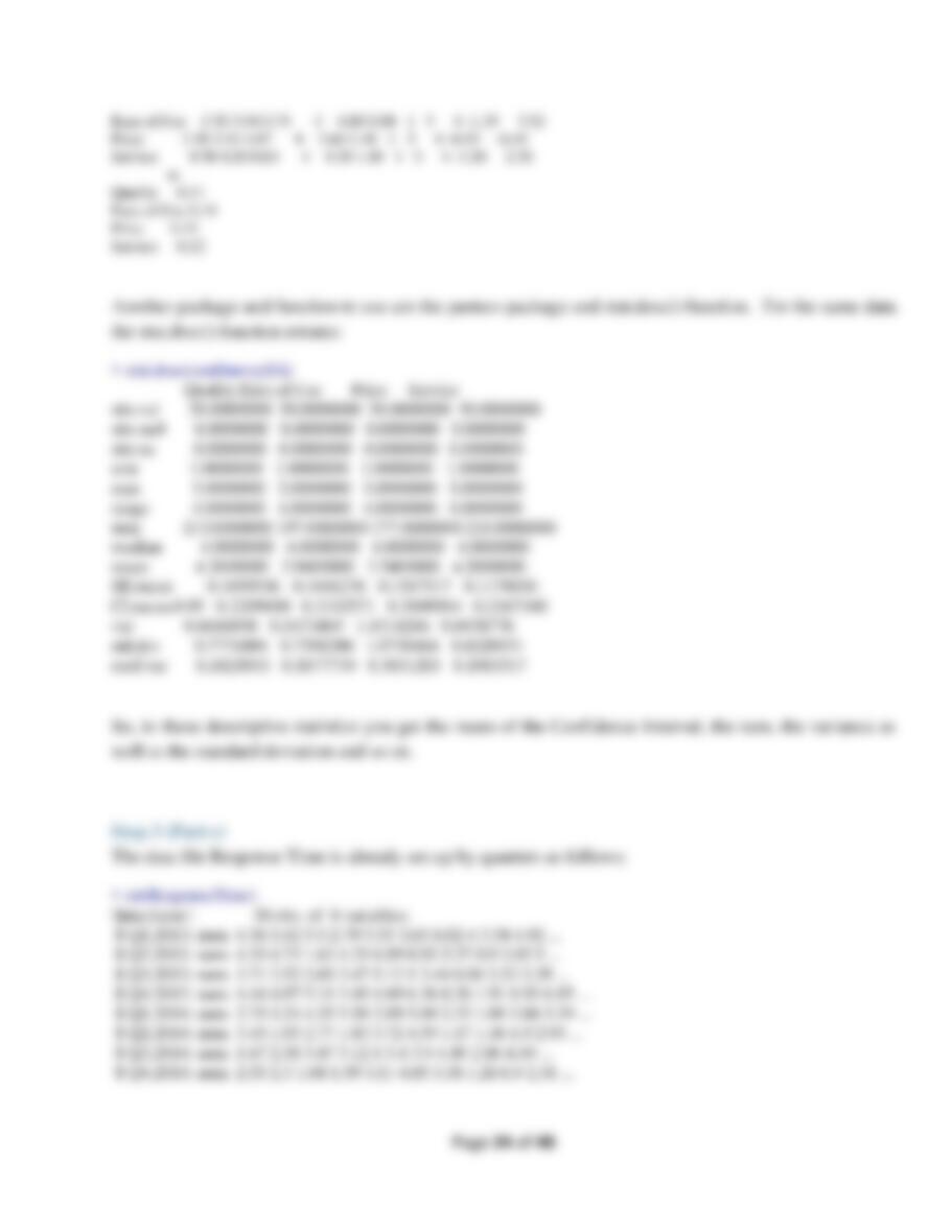
variables. Let’s consider one more of the data files in detail, i.e. the EmployeeRetention data file.
Using the str() function we get:
> str(EmployeeRetention)
‘data.frame’: 40 obs. of 7 variables:
$ YearsPLE : num 10 10 10 10 9.6 8.5 8.4 8.4 8.2 7.9 …
$ YrsEducation: int 18 16 18 18 16 16 17 16 18 15 …
$ College.GPA : num 3.01 2.78 3.15 3.86 2.58 2.96 3.56 2.64 3.43 2.75 …
$ Age : int 33 25 26 24 25 23 35 23 32 34 …
$ Gender : Factor w/ 2 levels “F“,”M”: 1 2 2 1 1 2 2 2 1 2 …
$ College.Grad: Factor w/ 2 levels “N“,”Y”: 2 2 2 2 2 2 2 2 2 1 …
$ Local : Factor w/ 2 levels “N”,“Y”: 2 2 1 2 2 2 2 2 2 2 …
where we have 40 observations for the 7 listed variables. Gender, College Grad, and Local are all listed
as “Factor” variables. This is the same as a categorical variable. If you are not familiar with different
data types you should take some time to look into this. One source you can use is:
https://www.tutorialspoint.com/r/r_data_types.htm.
Chapter 2 – Optional
Step 1
Find the total number of responses to each level of the surveys, Dealer and End-User Satisfaction, across
all regions for each year.
To do this we’ll need to subset the data by level and by year. Subsetting data is a standard part of data
analysis. As you will find with most things in R there are many ways of doing this. You can find lots of
information about this online. For example, because the data is essentially in the format of a matrix you
could use row and column numbers – if you know those. You can also use variable names or values.
For example,
> y2010 <- DealerSatisfaction[ which(DealerSatisfaction$Year == 2010), ]
establishes a new data object “y2010” and redirects observations from the DealerSatisfaction data file
into it in which the Year equals 2010. We can see the contents of “y2010” be just typing it on the
command line in the Console.
> y2010
Region Year L0 L1 L2 L3 L4 L5 Count

Page 6 of 48
1 <NA> 2010 1 0 2 14 22 11 50
6 SA 2010 0 0 0 2 6 2 10
11 EU 2010 0 0 1 3 7 4 15
16 PA 2010 0 0 1 2 2 0 5
Things to note include the syntax for the data filename and variable separated by a $, e.g.
DealerSatisfaction and Year as DealerSatisfaction$Year. To designate the test for “equals” use a double
==. You can use this syntax to find all the data required for this step. One of the really nice things
about RStudio is that you can move between commands you have used by the “up” and “down” arrows
on your keyboard. So, to go to the next year you only need to use the up arrow twice to go to the
command to subset the data and then change the year to 2011 to get the answers for the next year, and so
on. When you get to the part that asks for this data for End-User Satisfaction you just need to use the up
arrow appropriately and change the file name.
DO NOT forget to change the data object name for each command you use to store your results in. If
you do not change the data object name you will be continuously writing over your previous results.
To find the sum by year and return the value use the information you got before and sum, e.g.:
> y2010L0 <- sum(y2010[,3])
> y2010L0
[1] 1
That is, the sum for the year 2010 for all regions is 1. You can do this for all the instances you need to.
Choose data object names that make sense so that as you need them you can easily find them again and
again.
Keep in mind that R uses typical matrix notation, i.e. [rows, columns]. So you can always find the value
in an element in a matrix by its [row, column] designation.
Step 2
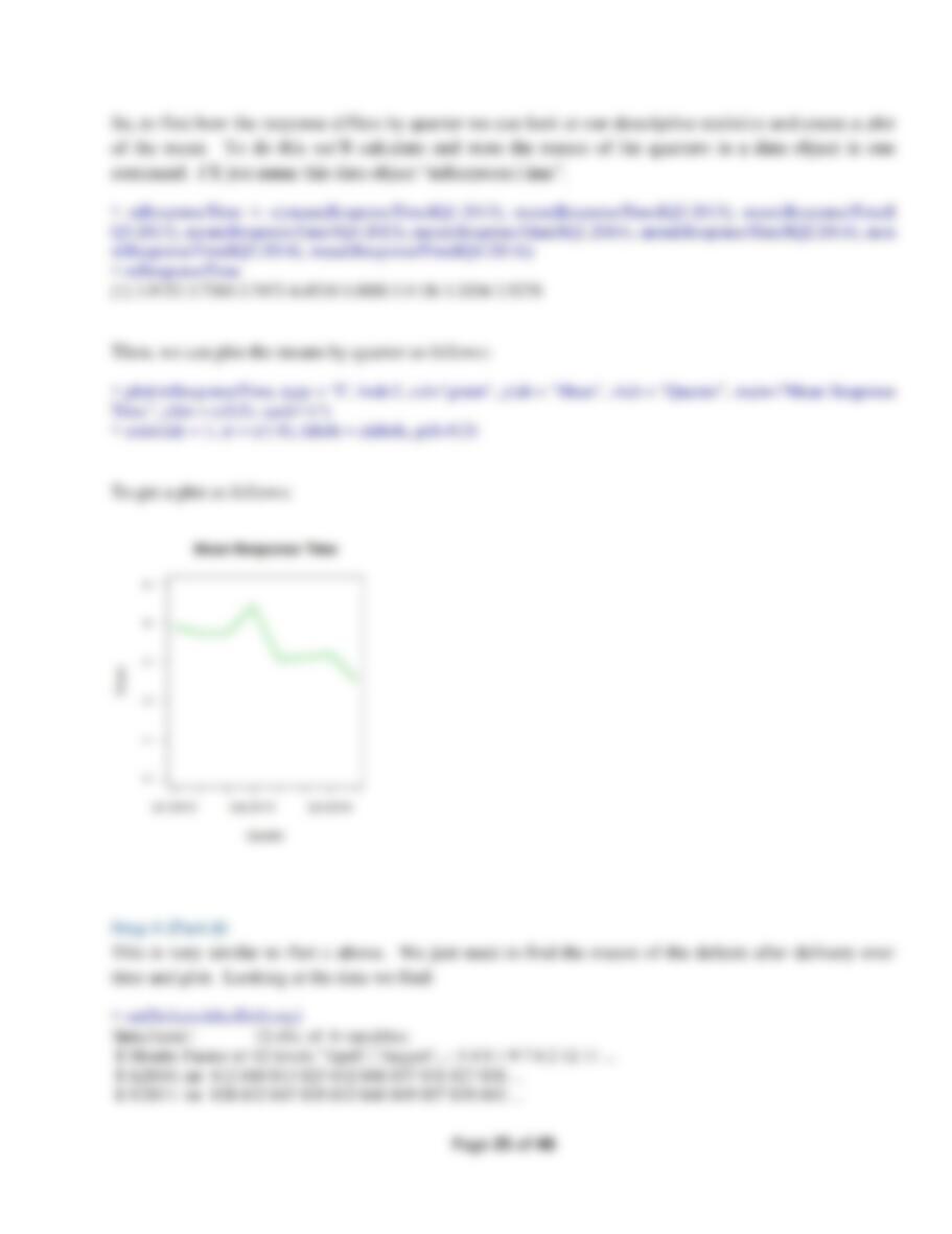
Find the number of failures in the Mower Test.
When the author completed this in Excel he just used the “COUNTIF” function for each column of his
spreadsheet Mower Test. This will take a bit more syntax in R but is relatively easy using the sapply()
function. There is actually a whole family of “apply” functions; e.g. apply, sapply, lapply, etc. All are
helpful in their way so check them out, e.g. in the answer at
http://stackoverflow.com/questions/3505701/r-grouping-functions-sapply-vs-lapply-vs-apply-vs-tapply–
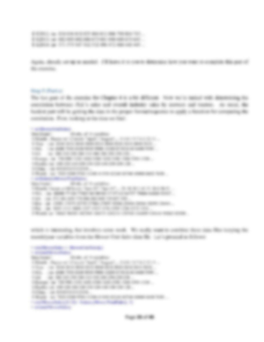
vs-by-vs-aggrega. For our question, we’ll use sapply() and the data file MowerTest but exclude the first
column which is the variable “Observations”. We’ll return the values of “Pass” and “Fail” as a table for
each of the Samples 1 through 30. The syntax we’ll use is:
> y <- t(sapply(MowerTest[-1], function(x) table(factor(x, levels = c(“Pass”, “Fail”)))))
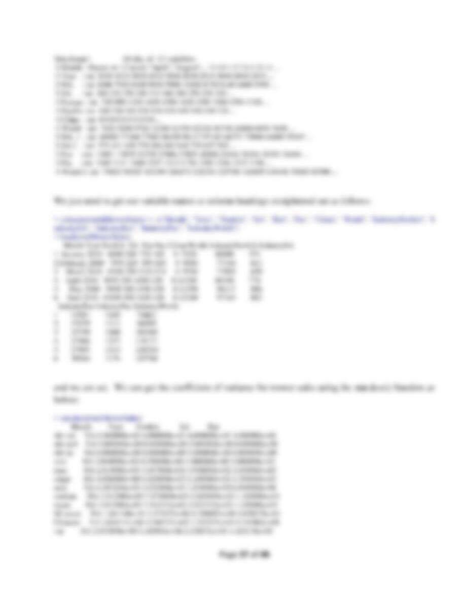
for which y returns:
> y
Pass Fail
Sample.1 97 3
Sample.2 96 4
Sample.3 99 1
Sample.4 100 0
Sample.5 99 1
Sample.6 95 5
Sample.7 98 2
Sample.8 99 1
Sample.9 100 0
Sample.10 98 2
Sample.11 98 2
Sample.12 97 3
Sample.13 97 3
Sample.14 99 1
Sample.15 99 1
Sample.16 98 2
Sample.17 98 2
Sample.18 97 3