cover page
Module 040
Inequality Analysis
The Gini Index

Inequality Analysis
The Gini Index
by
Lorenzo Giovanni Bellù, Agricultural Policy Support Service, Policy Assistance Division, FAO,
Rome, Italy
Paolo Liberati, University of Urbino, “Carlo Bo”, Institute of Economics, Urbino, Italy
for the
Food and Agriculture Organization of the United Nations, FAO
About EASYPol
EASYPol is a an on-line, interactive multilingual repository of downloadable resource materials for
capacity development in policy making for food, agriculture and rural development. The EASYPol home
page is available at: www.fao.org/tc/easypol.
EASYPol has been developed and is maintained by the Agricultural Policy Support Service, Policy
Assistance Division, FAO.
The designations employed and the presentation of the material in this information product do not imply
the expression of any opinion whatsoever on the part of the Food and Agriculture Organization of the
United Nations concerning the legal status of any country, territory, city or area or of its authorities, or
concerning the delimitation of its frontiers or boundaries.
© FAO December 2006 : All rights reserved. Reproduction and dissemination of material contained on
FAO’s Web site for educational or other non-commercial purposes are authorized without any prior
written permission from the copyright holders provided the source is fully acknowledged. Reproduction of
material for resale or other commercial purposes is prohibited without the written permission of the
copyright holders. Applications for such permission should be addressed to: copyright@fao.org.

Inequality Analysis: The Gini Index
Table of contents
1. Summary………………………………………………………………………1
2. Introduction……………………………………………………………………1
3. Conceptual background ……………………………………………………..2
3.1 The Gini Index ………………………………………………………………. 2
3.2 The generalised Gini Index (Gv)………………………………………….. 6
4. A step-by-step procedure to calculate the Gini Index ………………….9
4.1 The Gini Index ………………………………………………………………. 9
4.2 The generalised Gini Index………………………………………………. 11
5. A numerical example of how to calculate the Gini Index…………….12
5.1 The standard Gini Index with the Lorenz derivation…………………. 12
5.2 The standard Gini Index with the covariance formula ………………. 13
5.3 The generalised Gini Index………………………………………………. 13
6. The main properties of the Gini Index…………………………………..14
7. Lorenz intersection and the Gini Index………………………………….16
8. A synthesis of the main properties of the Gini Index and of its
generalised version …………………………………………………………18
9. Readers’ notes ……………………………………………………………..18
9.1 EASYPol links ………………………………………………………………. 18
10. Appendix I – Alternative ways to calculate the Gini Index…………..20
The geometrical derivation of the Gini Index and an alternative formula … 20
10.1 The Gini Index with the covariance formula ………………………….. 21
10.2 The main properties of the Gini Index…………………………………. 22
11. References and further reading…………………………………………..24
Module metadata……………………………………………………………………25

Inequality Analysis: The Gini Index
1
1. SUMMARY
This tool addresses the most popular inequality index, the Gini index. It discusses its
characteristics and the link with another popular graphical tool of representing
inequality, the Lorenz Curve. Extended version of the Gini Index with different
weighting schemes are also discussed. The use of the Gini Index and of its generalised
versions is explained through a step-by-step procedure and numerical examples.
2. INTRODUCTION
Objectives
The objective of this module is to introduce readers to the use of both the Gini Index
and the Generalised Gini Index, to compare income distributions and to discuss their
relative merits as well as their relative disadvantages.
Target audience
This module targets current or future policy analysts who want to increase their
capacities in analysing impacts of development policies on inequality by means of
income distribution analysis. On these grounds, economists and practitioners working in
public administrations, in NGOs, professional organisations or consulting firms will
find this helpful reference material. In addition, academics may find this material useful
to support their courses in Cost-Benefit Analysis (CBA) and development economics.
Furthermore, users can use this material to improve their skills in CBA and complement
their curricula.
Required background
Users should be familiar with basic notions of mathematics and statistics. In addition
they should have mastered the concepts of:
Income distribution and income inequality
Lorenz Curves
Inequality aversion.
Links to relevant EASYPol modules, further readings and references are included both
in the footnotes and in section 9 of this module1.
1 EASYPol hyperlinks are shown in blue, as follows:
a) training paths are shown in underlined bold font;
b) other EASYPol modules or complementary EASYPol materials are in bold underlined italics;
c) links to the glossary are in bold; and
d) external links are in italics.

EASYPol Module 040
Analytical Tools
2
3. CONCEPTUAL BACKGROUND
The Gini Index is an inequality measure that is mostly associated with the descriptive
approach to inequality measurement. Lambert (1993) provides a summary of the
analytical basis to link the Gini Index with social welfare functions, thus moving the
Gini Index into the field of welfare analysis. In what follows, we will be mostly
confined to the descriptive approach, leaving the welfare approach for more advanced
tools.
The Gini Index is a complex inequality measure2 and, as with many inequality
measures, it is a synthetic index. Therefore, its characteristic is that of giving summary
information on the income distribution and that of not giving any information about the
characteristics of the income distribution, like location and shape.
With regard to the Gini Index, we apply the logic of the inequality axioms3, as long as
axioms are eligible criteria to evaluate the indicator performances.
3.1 The Gini Index
The Gini Index was developed by Gini, 1912, and it is strictly linked to the
representation of income inequality through the Lorenz Curve. In particular, it measures
the ratio of the area between the Lorenz Curve and the equidistribution line
(henceforth, the concentration area) to the area of maximum concentration.
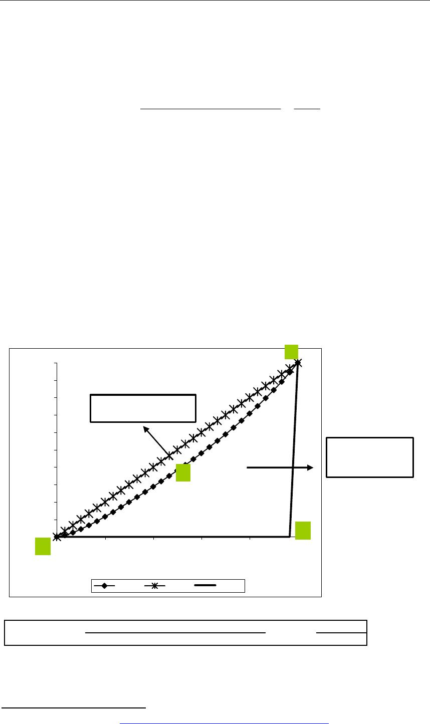
Figure 1 provides the visual representation of these areas, by drawing three
Lorenz Curves from three hypothetical income distributions, labelled A, B and C. The
shape of the Lorenz Curve based on income distribution A is the standard Lorenz Curve
we find (you find) when analysing actual income distributions. The Lorenz Curve of
income distribution B is an extreme case where all incomes are equal. In this case, the
Lorenz Curve is also called the equidistribution line. Finally, the Lorenz Curve of
income distribution C is another extreme case where all incomes are zero except for the
last one.
In Figure 1, as OP is the equidistribution line, ORP is the area defined by the
Lorenz Curve of the standard income distribution and the equidistribution line, what we
called the concentration area. Finally, OPQ is the area of maximum concentration, i.e.
the area between the Lorenz Curve of income distribution C and the equidistribution
line.
It should be clear that the equidistribution line OP and the area OPQ represent the
extreme values that the concentration area can assume in a Lorenz Curve representation.
Either this area is zero (as in the case of the equidistribution line of distribution B) or
this area is at its maximum (in the case of distribution C). For a standard income
distribution, the concentration area would be some way between zero and the area of
maximum concentration, as in Figure 1.
2 See EASYPol Module 080: Policy Impacts on Inequality: Simple Inequality Measures.
3 As discussed in EASYPol Module 054: Policy Impacts on Inequality: Inequality and Axioms for
its Measurement.
Inequality Analysis: The Gini Index
3
Now, the Gini Index measures the ratio of the concentration area to the maximum
concentration area. Therefore, in Figure 1:
[1]
OPQ
ORP
G== areaion concentrat maximum
areaion concentrat
As the maximum concentration area is obtained by a distribution where total income is
owned by only one individual, the Gini Index G, in general, measures the distance from
the area defined by any standard income distribution to the area of maximum
concentration.
It is now important to understand how the formula in Figure 1 can be applied in
practical terms. Let us start from the denominator of G. We have already explained4
that the maximum coordinates of the Lorenz Curve are at the point (1,1). The area
OPQ, therefore, must be a triangle with base length of 1 and height length of 1. Its area
is therefore equal to ½. The denominator of G is therefore ½.
Figure 1: The Lorenz Curve and the Gini Index
ORP
OP
Q
GINI = Concentration area =
Maximum concentration area
0.0
10.0
20.0
30.0
40.0
50.0
60.0
70.0
80.0
90.0
100.0
0.0 20.0 40.0 60.0 80.0 100.0
Cumulative proportion of population (%)
Cumulative proportion of income (%)
Dis_A Dis_B Dis_C
O
P
Q
ORP = Concentration
area
R
OPQ = Maximum
concentration
area
4 See EASYPol Module 000, Charting Income Inequality: The Lorenz Curve.
EASYPol Module 040
Analytical Tools
4
What about the numerator? Instead of calculating the concentration area directly, we
can exploit the fact that this area is given by the difference between the maximum
concentration area and the area under the Lorenz Curve (this latter being given by
ORPQ). The area under the Lorenz Curve is more easily calculated as follows.
5
First of all, let us recall the definition of the coordinates of the Lorenz Curve .
Given , it must be that:
n
yyy ≤≤≤ …
21
population of proportion cumulative
income of proportion cumulative
…
…
… 21
21
21
→=
→
+
+
+
=
+++
+
+
+
=
n
i
p
Y
yyy
yyy
yyy
q
i
i
n
i
i
with q0=p=0 and q
0 n=p=1.
n
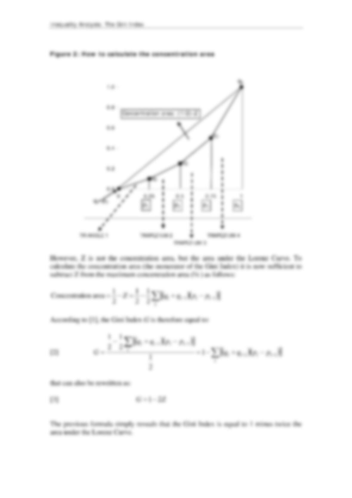
Now, the area ORPQ under the Lorenz Curve is the sum of the areas of a series of
polygons. Let us consider Figure 2, where a simplified Lorenz Curve is built for a
population of four individuals. The first polygon is a triangle (p q
o 1p1), the other three
polygons are rotated isosceles trapeziums. Each area can therefore be calculated
separately, and separate results added to get the value of the overall area. Let us define