A SIMPLE MODEL OF THE FIRM

The decision setting we will investigate can be described as

follows:

1. A firm produces a single good or service for a single market

with the objective of maximizing profit.

2. Its task is to determine the quantity of the good to produce

and sell and to set a sales price.

3. The firm can predict the revenue and cost consequences of its

price and output decisions with certainty.

Together these three statements fulfill the first four fundamental

decision making steps described in Chapter 1. Statement 1

specifies the setting and objective, statement 2 the firm’s

possible decision alternatives, and statement 3 (along with some

specific quantitative information supplied shortly) the link

between actions and the ultimate objective, namely, profit. It

remains for the firm’s manager to “solve” and explore this

decision problem using marginal analysis (steps 5 and 6).

Before turning to this task, note the simplifying facts embodied

in statement 1. Typically, a given firm produces a variety of

goods or services. Nonetheless, even for the multiproduct firm,

examining products one at a time has significant decision

advantages. For one thing, it constitutes an efficient managerial

division of labor. Thus, multiproduct firms, such as Procter &

Gamble, assign product managers to specific consumer

products. A product manager is responsible for charting the

future of the brand (pricing, advertising, promotion, and

production policies). Similarly, most large companies make

profit-maximizing decisions along product lines. This product–

by-product strategy is feasible and appropriate as long as the

revenues and costs of the firm’s products are independent of one

another. (As we shall see in Chapters 3 and 6, things become

more complicated if actions taken with respect to one product

affect the revenues or costs, or both, of the firm’s other

products.) In short, the firm can maximize its total profit by

separately maximizing the profit derived from each of its

product lines.

A Microchip Manufacturer

As a motivating example, let’s consider a firm that produces and

sells a highly sophisticated microchip. The firm’s main problem

is to determine the quantity of chips to produce and sell (now

and in the immediate future) and the price. To tackle this

problem, we begin by examining the manager’s basic objective:

profit.

A simple accounting identity states that profit is the difference

between revenue and cost.

In algebraic terms, we have (π =R – C), where the Greek letter

Pi (π) stands for profit. To see how profit depends on the firm’s

price and output decisions, let’s examine the revenue and cost

components in turn.

REVENUE The analysis of revenue rests on the most basic

empirical relationship in economics: the law of demand.

This law states:

(All other factors held constant, the higher the unit price of a

good, the fewer the number of units demanded by consumers

and, consequently, sold by firms.)

Suppose the leading firms raise their chip prices due to the

increased cost of silicon. According to the law of demand, the

industry’s total sales of chips will fall. Let’s suppose that

currently there is a stable pattern of (different) prices and market

shares for the leading firms in the industry. Consider what

would happen if one of the firms unilaterally instituted a

significant reduction in the price of its chips. The law of demand

predicts that its microchip sales would increase.

The sources of the increase are threefold:

(1) increased sales to the firm’s current customers,

(2) sales gained from competing suppliers, and

(3) sales to new buyers.

Of course, each of these factors might be important to a greater

or lesser degree.

Figure 2.2 graphically illustrates the law of demand by depicting

the individual firm’s downward-sloping demand curve. The

horizontal axis lists the quantity of microchips demanded by

customers and sold by the firm each week. For convenience, the

quantity of chips is measured in lots consisting of 100 chips.

The vertical axis lists the price per lot (measured in thousands of

dollars) charged by the firm. Three particular points along the

downward-sloping demand curve are noted. Point A

corresponds to a quantity of 2 lots and a price of $130,000; this

means that if the firm charges $130,000 per lot, its weekly sales

will be 2 lots (or 200 chips). If the firm cut its price to $100,000,

its sales would increase to 3.5 lots (point B). A dramatic

reduction to a price of $50,000 would increase sales to 6 lots

(point C). Thus, the demand curve shows the firm’s predicted

sales over a range of possible prices. The downward slope of the

curve embodies the law of demand: A lower price brings forth

an increased quantity of sales.

The firm uses the demand curve as the basis for predicting

the revenue consequences of alternative output and pricing

policies.

Quite simply, the demand curve allows the firm to predict its

quantity of sales for any price it charges. In turn, revenue can be

computed as the product of price and quantity. The most useful

way to begin the revenue estimation task is to work with the

mathematical representation of the demand curve. An algebraic

representation of the demand curve

Q = 8.5 – 0.05P

Where Q is the quantity of lots demanded per week and P

denotes the price per lot (in thousands of dollars). In this form,

the demand equation predicts the quantity of microchips sold at

any given price. For instance, if P equals $50 thousand, then,

according to Equation 2.1, Q equals 6 lots (point C in the

figure); if P equals $130 thousand, Q equals 2 lots, and so on.

For any price the firm charges, the demand equation predicts

the resulting quantity of the good that will be sold.

With a bit of algebraic rearrangement, we can derive an

equivalent version P = 170 – 20Q

This price equation usually is referred to as the firm’s inverse

demand equation.

The demand equation or the inverse demand equation contains

all the information the firm needs to predict revenue.

However, before launching into the revenue analysis, we

should pause to make two points.

1- First, the demand equation furnishes a quantitative

snapshot of the current demand for the firm’s product as it

depends on price. Of course, many other factors, including

competing firms’ products and prices and the general

strength of the computer industry, affect the firm’s chip

sales. The demand prediction of Equation 2.1 is based on

the current state of these factors. If economic conditions

change, so too will the firm’s sales at any given price; that

is, Equation 2.1 would no longer be a valid representation

of the new demand conditions. Keep in mind that our use

of the demand equation takes other demand-relevant

factors as given, that is, unchanged.

2- The second point is that we view the demand curve as

deterministic; that is, at any given price, the quantity sold

can be predicted with certainty. For a given price,

Let’s use Equation 2.2 to predict the revenues generated by

alternative sales policies of the microchip manufacturer.

Figure 2.3 contains the pertinent information and provides a

graph of revenue.

Column 1 of the tabular portion lists a spectrum of possible

sales quantities ranging from 0 to 8.5 lots. It will be convenient

to think of the sales quantity, Q, as the firm’s decision variable,

that is, the variable it explicitly chooses. For each alternative

choice of Q, column 2 lists the corresponding sales price

obtained from Equation 2.2. (Be sure you understand that the

firm cannot set both Q and P independently. Once one is set, the

other is determined by the forces of demand embodied in the

demand equation.) Finally, column 3 lists the resulting revenue

earned by the firm, where revenue is defined as R = P x Q.

From the table, we observe that revenue is zero when sales are

zero (obviously). Then as Q increases, revenue initially rises,

peaks, and eventually begins to fall, finally falling to zero at Q =

8.5 lots. (Note that to sell 8.5 lots, the requisite sales price from

Equation 2.2 is zero; that is, the lots would have to be given

away.) In short, the law of demand means that there is a

fundamental trade-off between P and Q in generating revenue.

An increase in Q requires a cut in P, the former effect raising

revenue but the latter lowering it. Operating at either extreme—

selling a small quantity at high prices or a large quantity at very

low prices—will raise little revenue.

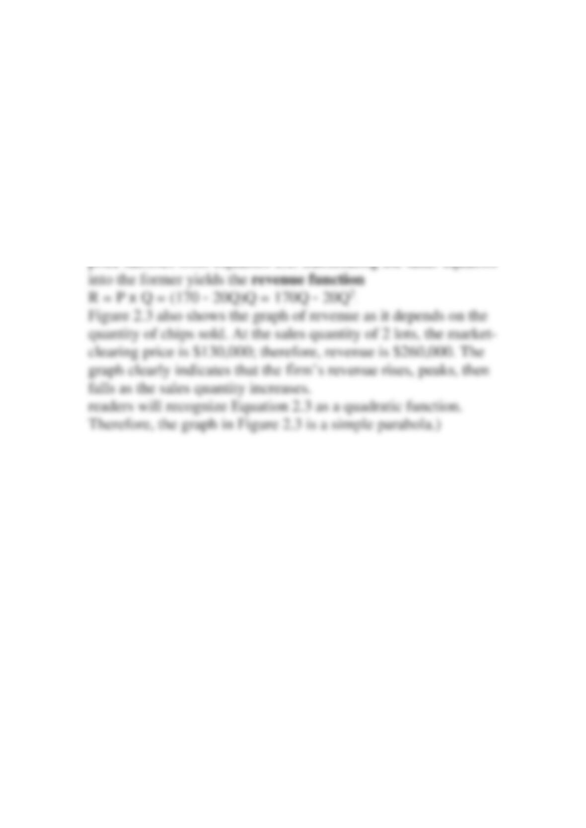
The revenue results in Figure 2.3 can be obtained more directly

using basic algebra. We know that and that the market-clearing