A Crash Course in Statistics at FIU – The One Way ANOVA (#3)
So you took Stats I and Stats II at FIU and passed. But do you remember what you did, how you
did it, and why you did it? If you need some basic statistic reminders for the One Way ANOVA,
then this is the lecture for you! I am going to talk about a One Way ANOVA example in this
document that corresponds to the same example you saw in the Descriptive Statistics Crash Course
(#1) and t-Test Crash Course (#2) where participants were asked to recall how much money they
spent on textbooks the prior semester. However, for this ANOVA crash course, we are going to
add a third condition: control (a third group of participants who do not see any prior book recall
amounts on the list). As you can see here, we have ONE independent variable (hence the One Way
ANOVA), but here we have three levels (or three conditions): High, Low, and Control. The good
news is that this mini-lecture will sum up the basics of the ANOVA for you as we look at this
study, but you can find additional information about the ANOVA in your textbooks. On the final
pages of this document are several questions based on this crash course. Answer these questions,
and then go into your “Crash Course in Statistics – The One Way ANOVA Quiz #3” in your
Canvas assessments menu and copy over your answer. Each Crash Course Quiz counts 5 points.
How, when, and why do a One Way ANOVA?
Before we get to the example, let me give you some basic information about the One Way
ANOVA. Do you recall the t-Test, where we compared two means to see whether and in what
direction the means differed? Well, a One Way ANOVA is very similar, but here we compare
three or more means to see if they differ significantly from one another. In this analysis, we
need three pieces of information: 1) the means for each of the three groups (descriptive
statistics), 2) the One Way ANOVA information itself, and 3) post hoc tests.
1). Once again, remember that a mean is the average score for that condition. That is, you add
up all of the scores in a condition and divide by the number of total scores to arrive at the
average. Since a One Way ANOVA looks at three or more different conditions, we have at
least three means: one for each condition. The means here (plus the standard deviation, which
we will talk about in the lecture) are descriptive statistics. That is, they help describe the data.
2). The One Way ANOVA information itself is a test of inferential statistics. That is, we infer
significant differences between the three or more groups. When writing it out, you will see a
very common layout for the One Way ANOVA, something like: F(2, 134) = 2.61, p = .021.
The F tells you this is a One Way ANOVA. The 2 and 134 tells us our degrees of freedom
(more on that in out lecture). The 2.61 is the actual number for the One Way ANOVA. The p
indicates whether it is significant (if it is less than .05, then it is significant).
3). Finally, we have to consider post hoc tests. You might recall using the Tukey post hoc test
in the past, but do you remember why you used it? Take a step back and think about the t-Test,
which looked at two means: Mean A and Mean B. If Mean A is 4.56 and Mean B is 7.67 and
your t-Test is significant (that is, p is less than .05), then you simply compare the two means to
see which is higher: Mean A or Mean B. Here, Mean B is clearly higher (7.67 is higher than
4.56), and since the t-Test is significant then Mean B is significantly higher than Mean A. But
when we have three levels to our independent variable, we are now dealing with three means:
Mean A, Mean B, and Mean C. Let’s say Mean A is 4.56, Mean B is 7.67, and Mean C is 6.21.
If our One Way ANOVA is significant (that is, it is less than .05), we know the means differ.

The question is, which of the three means differ? Does Mean A differ from Mean B? Does
Mean B differ from Mean C? Does Mean A differ from Mean C? Or there might be other
combinations. Maybe Mean A and Mean C do not differ from each other, but both are
significantly lower than Mean B. Unlike the t–Test, we don’t know which of the three means
differ, which is why we run a post hoc test (like Tukey) to compare Mean A to Mean B, and
Mean A to Mean C, and Mean B to Mean C. It runs all of those analyses for us in one test. So
you might wonder, “Why not just run three t-Tests, with one t-Test comparing Mean A to
Mean B, a second t-Test comparing Mean B to Mean C, and a third t-Test comparing Mean B
to Mean C.?” Well, you could actually do that, but we run into a Type I error. That is, the more
tests we run, the greater the chance one of them will be significant. If we run three t-Tests, we
open up the chance of one of them being falsely positive. With the One Way ANOVA, we just
run the one test to compare the three means (note that the post hoc tests are still a part of the
One Way ANOVA – it compares the three means under the umbrella of the One Way ANOVA
test).
Like the t-Test, we run a One Way ANOVA only under certain conditions.
First, our dependent variable (the variable we measure) must be continuous / scaled. That
is, the DV has to be along a scale. For example, it can be an attitude (“On a scale of 1 to 9,
how angry are you?”), a time frame (“How quickly did the salesperson help the customer
on a scale of zero seconds to a thousand seconds?”), or money estimation (“How much do
you recall spending on textbooks last semester?”). We call these interval or ratio scales,
which means we can use a t-Test or ANOVA. We CANNOT run a One Way ANOVA on
categorical data. That is, if we have a yes / no question (“Are you lonely: Yes or No”) or a
category based question (“What is your favorite food: hamburgers, pizza, salad, or
tacos?”), then we cannot run a One Way ANOVA. These latter questions are based more
on choice of option rather than an actual rating scale, and thus we cannot use a One Way
ANOVA on them.
Second, we run a One Way ANOVA when we have only one independent variable and that
independent variable has at least three conditions (Note: it can have more than three levels,
but you still only have one independent variable). That is, we compare the means from
Condition A, Condition B, and Condition C. If our One Way ANOVA is significant (p <
.05), then we look at our post hoc tests to see which means differ. “The One Way ANOVA
was significant, F(2, 134) = 2.61, p = .021. Tukey post hoc tests showed that Condition A
(mean = 48.38) was significantly lower than Condition B (mean = 63.25). In addition,
Condition C (mean = 48.88) was significantly lower than Condition B. However, Condition
A did not differ significantly from Condition C.”
Let’s see how this looks using the textbook money example.
Textbook Study – How Much Did You Spend On Textbooks (High, Low, or Control)
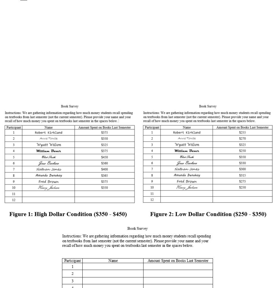
Recall the basic set-up for our money spent on textbooks. Researchers ask participants to recall
how much they spent on textbooks the prior semester, and has each participant write their
answer on a survey sheet. In two conditions, the first ten answer slots are already filled in,
presumably by other respondents. However, the researcher actually completed those ten slots,
and manipulated the dollar amounts so that in in the High Dollar Condition, the dollar amounts
ranged from $350 to $450 (Figure 1). In the Low Dollar Condition, amounts ranged from $250
to $350 (Figure 2). In our new study, the researcher provides a third condition in which there
are no prior dollar amounts on the list (Control Condition – Figure 3). Using psychological
principles based on conformity and informational social influence (e.g. participants relying on
the behavior of other individuals when they lack a clear memory), the researcher predicts that
those in the High Dollar Condition will recall spending more money on textbooks the prior
semester than those in the Low Dollar Condition, with those in the Control condition providing
a dollar amount somewhere in the middle.
Here, the independent variable is Dollar Condition (High versus Low versus Control) while the
dependent variable is the amount of money participants recall spending on textbooks (in $).
Imagine we have eight real participants in the High Dollar Condition, eight real participants in
the Low Dollar Condition, and eight real participants in the Control Condition (and no, we are
not including the original researcher-completed dollar amounts on the sheet passed out by the
researcher in the High and Low Dollar Conditions, as those are not real participants!).
Figure 3: No Prior Dollar Amount Condition
Consider the data:
Condition A (High)
Condition B (Low)
Condition C (Control)
350
275
300
400
350
325
375
325
300
350
275
300
300
250
275
325
260
350
300
300
325
300
315
275
∑A = 2700
∑B = 2350
∑C = 2450
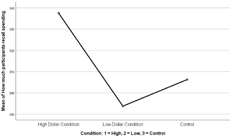
Mean = $337.50
Mean = $293.75
M = $306.25
∑, or the symbol for Sigma, means “the sum of”. Thus ∑A is the sum of the scores for
Condition A. That is, 350 + 400 + 375 + 350 + 300 + 325 + 300 + 300 = 2700. There are eight
scores here, so we divide 2700 / 8 = 337.50, giving us our mean of $337.50 for Condition A
(High Dollar Condition). We do the same thing for Condition B (Low Dollar Condition),
giving us a mean of $293.75 (2350 / 8 = 293.75). Finally, we do the same thing for Condition
C (Control), giving us a mean of $306.25 (2450 / 8 = 306.25).
For the first part of our analysis, we compare the means. As you see, $293.75 in Condition B