LECTURE TEXT
First-order differential equations in chemistry
Gudrun Scholz •Fritz Scholz
Received: 7 August 2014 / Accepted: 13 September 2014 / Published online: 25 November 2014
ÓSpringer International Publishing 2014
Abstract Many processes and phenomena in chemistry,
and generally in sciences, can be described by first-order
differential equations. These equations are the most
important and most frequently used to describe natural
laws. Although the math is the same in all cases, the stu-
dent may not always easily realize the similarities because
the relevant equations appear in different topics and con-
tain different quantities and units. This text was written to
present a unified view on various examples; all of them can
be mathematically described by first-order differential
equations. The following examples are discussed: the
Bouguer–Lambert–Beer law in spectroscopy, time con-
stants of sensors, chemical reaction kinetics, radioactive
decay, relaxation in nuclear magnetic resonance, and the
RC constant of an electrode.
Keywords Differential equations Bouguer–Lambert–
Beer law Time constants Chemical kinetics
Radioactive decay Nuclear magnetic resonance RC
constant
Introduction
‘‘Differential equations are extremely important in
the history of mathematics and science, because the
laws of nature are generally expressed in terms of
differential equations. Differential equations are the
means by which scientists describe and understand
the world’’ [1].
The mathematical description of various processes in
chemistry and physics is possible by describing them with
the help of differential equations which are based on simple
model assumptions and defining the boundary conditions
[2,3]. In many cases, first-order differential equations are
completely describing the variation dyof a function y(x)
and other quantities. If yis a quantity depending on x,a
model may be based on the following assumptions: The
differential decrease of the variable yis proportional to a
differential increase of the other variable, here x, i.e.
–dy*dx. This decrease –dyshould depend on the
function yitself: –dy*ydx, and together with a so far
unknown constant a, results in the equation
dy¼aydxð1Þ
Thus follows the ordinary linear homogeneous first–
order differential equation:
dy
dxþay ¼0ð2Þ
The characteristics of an ordinary linear homogeneous
first–order differential equation are: (i) there is only one
independent variable, i.e. here x, rendering it an ordinary
differential equation, (ii) the depending variable, i.e. here y,
having the exponent 1, rendering it a linear differential
equation, and (iii) there are only terms containing the
Electronic supplementary material The online version of this
article (doi:10.1007/s40828-014-0001-x) contains supplementary
material, which is available to authorized users.
G. Scholz
Department of Chemistry, Humboldt-Universita
¨t zu Berlin,
Brook-Taylor-Str. 2, 12489 Berlin, Germany
F. Scholz (&)
Institute of Biochemistry, University of Greifswald,
Felix-Hausdorff-Str. 4, 17487 Greifswald, Germany
e-mail: fscholz@uni-greifswald.de
123
ChemTexts (2014) 1:1
DOI 10.1007/s40828-014-0001-x
variable yand its first derivative, rendering it a homoge-
neous first–order differential equation.
This equation can be solved when, e.g. the boundary
conditions are such that yvaries between y
0
and y, when x
varies between 0 and x. Following a separation of vari-
ables, the integration of Eq. 2gives:
dy
y¼adxð3Þ
Zy
y0
dy
y¼aZx
0
dxð4Þ
ln y
y0¼ax ð5Þ
y¼y0eax ð6Þ
Equation 6describes the exponential decrease of yas a
function of x.
This formalism will now be applied to some special
cases which occur frequently in chemistry, and finally all
discussed cases will be compared in a table.
The Bouguer–Lambert–Beer Law
The intensity of electromagnetic radiation (e.g. visible
light), i.e. exactly the radiant flux I(unit W, watt or J s
–1
,
joule per second), diminishes along the path length
xthrough a homogeneous absorbing medium (e.g. a col-
oured solution). Figure 1depicts a cuvette and the changes
in radiant flux along the optical path length.
The differential decrease –dIof radiant flux by passing
through the differential length increment dxis supposed to
be proportional to the actual value of Iat x
i
. To understand
this, we must consider the physical background of the
decrease of radiant flux: If the radiation is understood as a
flux of photons, the absorption of radiation is the loss of
photons due to their ‘‘capture’’ by absorbing particles
(molecules, atoms or ions) in the cuvette. Clearly, the
effectivity of capture must be proportional to the number of
particles per volume, i.e. their concentration cin mol L
–1
,
as the probability that a photon hits a particle will be
proportional to its concentration. However, not each hitting
leads to an absorption event (capture of a photon). To take
into account the probability that a collision of a photon
with a particle leads to its capture, one defines an effective
cross section of the particles. This cross section has the unit
of an area because one may understand it as an effective
target area for the photons in contrast to the geometric
target area which a particle exposes to the photon flux.
Instead of using the effective cross section, one may define
a constant j(Greek letter kappa) which theoretically can
have values between 0 and 1, giving the fraction of suc-
cessful absorption events. jis a value specific for the
particles and specific for the photon energy E
photon
, and
thus the frequency m(Greek letter nu) of the radiation, with
m=E
photon
/h(his the Planck constant
6.62606957(29) 910
–34
Js), and the wavelength k(Greek
letter lambda) with k¼hclightEphoton (clight being the
velocity of light in the respective medium).
From the preceding discussion follows that the differ-
ential equation
dIðxÞ¼IðxÞjcdxð7Þ
adequately describes the decrease of radiation flux. Since j
is specific for the energy of absorbed photons, this equation
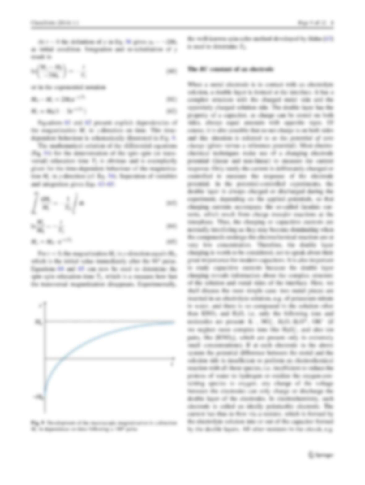
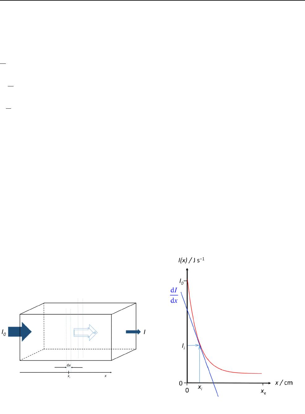
Fig. 1 Electromagnetic radiation is trespassing a cuvette filled with a
homogeneous absorbing medium. I0is the radiant flux before entering
the cuvette, Iis the radiant flux leaving the cuvette, dIis the
differential decrease of radiant flux by passing through the differential
length increment dxat xi
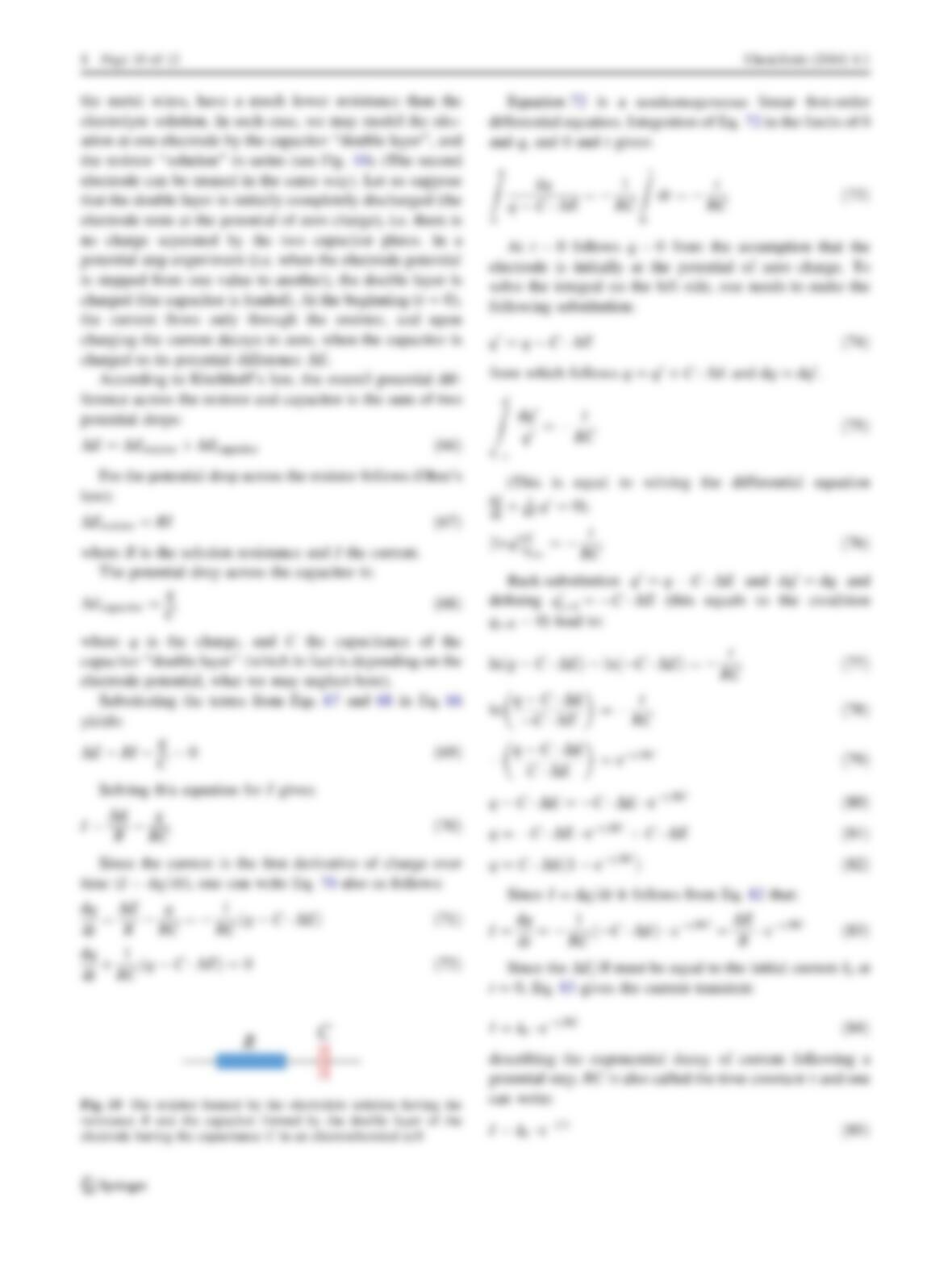
Fig. 2 The decay of radiation flux when passing through the
absorbing medium
1Page 2 of 12 ChemTexts (2014) 1:1
123
relates to monochromatic radiation (radiation with one
constant frequency, i.e. photon energy). The meaning of
Eq. 7can be understood with the help of Fig. 2:Ifxemarks
the overall length which the electromagnetic radiation
passes through the absorbing medium, and the intensity
(radiation flux) of the incident light is I0(at x¼0), then at
a path length xithe intensity of light will have dropped to Ii
and the slope of IðxÞ¼fðxÞ, i.e. dIðxÞ
dxwill be proportional
to Iiand jand c.
Integration of Eq. 7and some rearrangements have to be
performed as follows:
dIðxÞ
IðxÞ¼jcdxð8Þ
ZI
I0
dIðxÞ
IðxÞ¼jcZxe
0
dxð9Þ
ln I
I0¼jcxeð10Þ
ln I0
I¼jcxeð11Þ
log I0
I¼1
ln 10 jcxe0:4343jcxeð12Þ
The ratio log I0
Iis called absorbance A, and the product
0:4343jis called the molar absorption coefficient e(Greek
letter epsilon) or molar absorptivity. The path length of the
radiation xeis usually given the symbol l. The Bouguer–
Lambert–Beer Law is thus normally written as:
A¼ecl ð13Þ
Outside of this purely mathematical analysis, it needs
to be mentioned that Eq. 13 has a restricted range of
validity: it is a good description of real systems only
at low concentrations. At higher concentrations
(sometimes already above 10
–5
mol L
–1
) intermo-
lecular interactions of the absorbing particles, and
chemical equilibria can lead to deviations (apparent
variations of the molar absorption coefficient). Fur-
ther, another contribution to the absorption coeffi-
cient depends on the refractive index nof the
solution. Because the refractive index may signifi-
cantly vary with the concentration of the dissolved
analyte, it is not e, which is constant, but the molar
refraction and the term en=ðn2þ2Þ2should be used
instead of e[4].
The time constant of a sensor
Sensors measure a physical or chemical quantity and
transduce it to an output signal which is read, monitored
or stored. Possible physical quantities are temperature,
pressure, radiative flux, magnetic field strength, etc.
Chemical quantities are mainly concentrations and activ-
ities of molecules, atoms and ions. The recorded signals
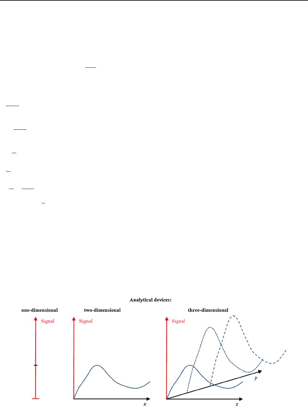
are usually voltages or currents. The most typical feature
of a signal is that the results are one dimensional, e.g. the
output signal is a single quantity, i.e. one measures only
that signal and not a dependence of that signal on another
given quantity. Most devices for chemical analysis pro-
duce two-dimensional read-outs, e.g. optical spectra in
which the absorbance is displayed as a function of
wavelength (E¼fðkÞ), voltammograms in which currents
are displayed as function of electrode potential or X-ray
diffractograms, in which the intensity of diffracted rays is
displayed as function of diffraction angle, etc. In modern
instrumentation, one has even expanded the
Fig. 3 A comparison of the three common dimensionalities of analytical devices
ChemTexts (2014) 1:1 Page 3 of 12 1
123
dimensionality to three, when, as an example, optical
spectra (E¼fðkÞ) (or mass spectra, i.e. ion intensities
versus the mass-to-charge ratio of ions) are displayed as a
function of elution time of a chromatogram. Figure 3
gives a comparison of the common dimensionalities of
analytical measurements.
Since any measurement needs time, there is nothing like
an instantaneous establishment of a signal. This is easy to
see when using a sensor, e.g. a pH electrode: There is
always a certain time period in which the reading changes
until we finally have the impression that a constant end
value is reached. The same is true also for two- or three-
dimensional measurements, but we cannot easily detect it
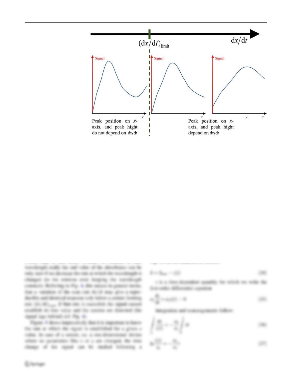
because the variation of the measured signal (e.g. the
absorbance) anyway changes as a function of the varied
quantities (e.g. the wavelength) and thus with time. Nor-
mally, the wavelength is changed with the so-called scan
rate dk=dt(rate of recording the spectrum), and generally
(see Fig. 4), the quantity xis varied with a scan rate dx=dt
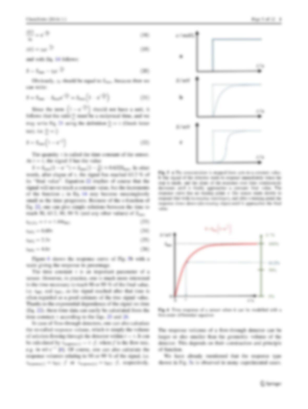
concentration step. The introduction of the sensor into a
solution can be regarded as a concentration step. Figure 5
depicts two different kinds of response of a sensor on a
concentration step.
Figure 5depicts two basic types of time responses of
sensors. The different sensor behaviours shown in B and C
can be modelled with the help of different differential
equations. Whereas the response curve shown in B can be
modelled with a first-order differential equation; the curve
shown in C needs higher-order differential equations [5]. At
this point, it is necessary to note that it is impossible to realize
a concentration step with infinite rate of concentration rise, as
shown in Fig. 5a. This means, when the temporal response
properties of a sensor are studied, this concentration rise has
to be much quicker than the response of the sensor. Further,
also the response shown in Fig. 5b is to some extend an
idealization, and in reality there may be always a sluggish
response at the start, but it may be on such short time scale
that it escapes our recognition. The response curve shown in
Fig. 4 Possible distortion of a
spectrum when the rate of
changing xwith time above a
limiting value ðdx=dtÞlimit
1Page 4 of 12 ChemTexts (2014) 1:1