Unlock document.
This document is partially blurred.
Unlock all pages and 1 million more documents.
Get Access

1
Solutions To Problems of Chapter 5
5.1. Show that the gradient vector is perpendicular to the tangent at a point
of an isovalue curve.
Solution: The differential of the cost function, J(θ), at a point θ(i), is
given by
5.2. Prove that if ∞
X
i=1
µ2
i<∞,
∞
X
i=1
µi=∞,
the steepest descent scheme, for the MSE loss function and for the iteration-
dependent step size case, converges to the optimal solution.
i
X
k=1
µ2
k∇TJ(θ(k−1))∇J(θ(k−1))−
2
i
X
k=1
µk(θ(k−1) −θ∗)T∇J(θ(k−1)).
(θ(i)−θ∗)T(θ(i)−θ∗)−(θ(0) −θ∗)T(θ(0) −θ∗)≤A
i
X
k=1
µ2
k−
2
i
X
k=1
µk(θ(k−1) −θ∗)T∇J(θ(k−1)),
5.3. Derive the steepest gradient descent direction for the complex-valued case.
Solution: We know from the text that
J(θ+ ∆θ) = J(θr,θi)+∆θT
r∇rJ(θr,θi) +
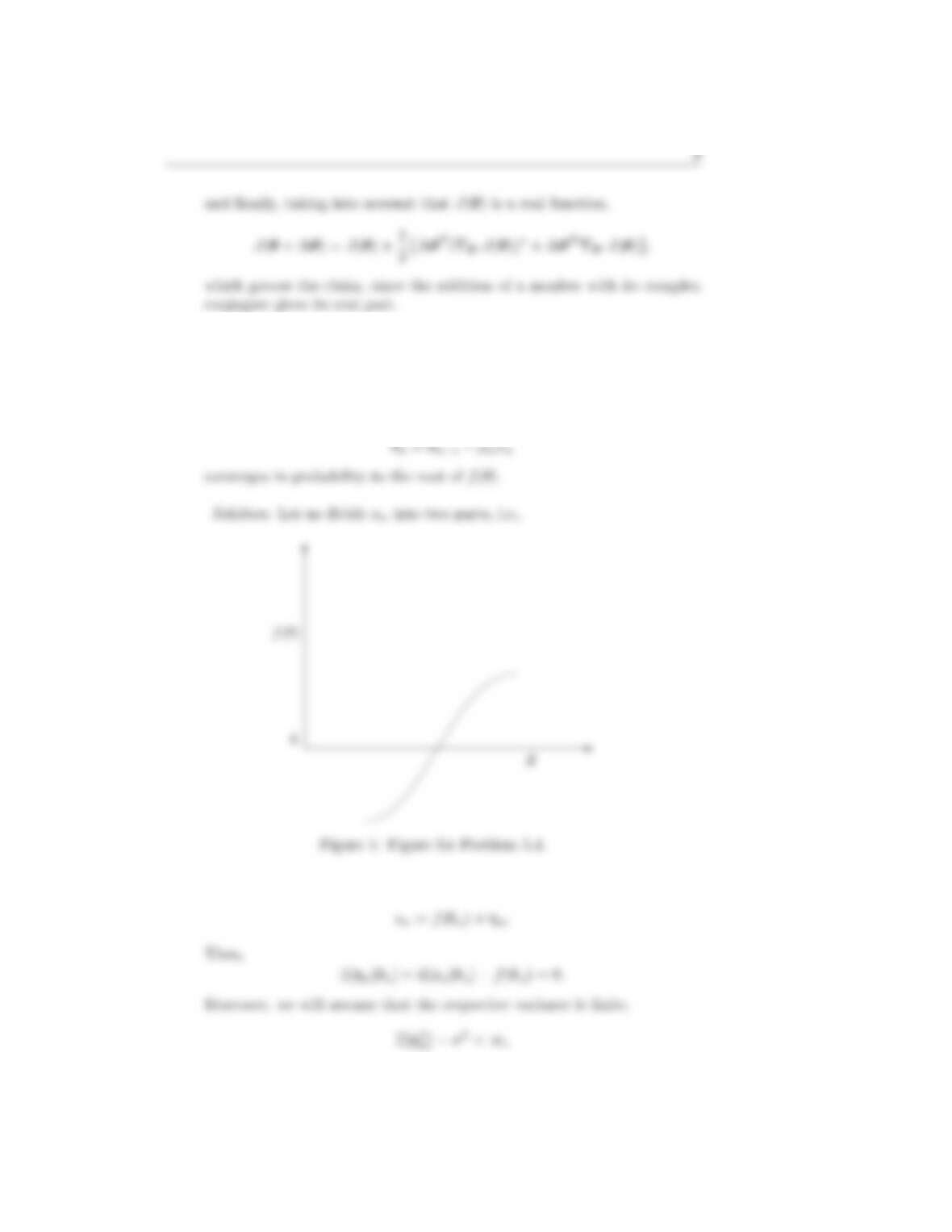
5.4. Let θ,x be two jointly distributed random variables. Let also the function
(regression)
f(θ) = E[x|θ],
assumed to be an increasing one. Show that under the conditions in (5.29)
the recursion
4
and also we assume that ηnand θnare independent. Let θ∗be a root.
Then, we form
θn−θ∗=θn−1−θ∗−µnf(θn−1)−µnηn.
Taking the expectation of the square we get
i=1
Assume now that
E[f2(θn−1)] ≤b < ∞.
Then we obtain the following,
E[(θn−θ∗)2]−E[(θ0−θ∗)2≤(b+σ2)
n
X
µ2
i−
n
X
provided a single root exists.
Thus,
f(θ)(θ−θ∗)≥0,(2)
and hence,
E[(θi−θ∗)f(θi)] ≥0.
5.5. Show that the LMS algorithm is a nonlinear estimator.
Solution: Consider the basic LMS recursion
θn=θn−1+µxnen
5.6. Show equation (5.42).
Solution: Our starting point is
Σc,n =Σc,n−1−µΣxΣc,n−1−µΣc,n−1Σx
5.7. Derive the bound in (5.45).
Hint: Use the well known property from linear algebra, that the eigenval-
ues of a matrix, A∈Rl×l, satisfy the following bound,
max
1≤i≤l|λi| ≤ max
1≤i≤l
l
X
|aij |:= kAk1.
i
j=1
This is a suffcient condition for stability and guarantees that all eigenval-
ues of Ahave magnitude less than one, or
l
X
5.8. Gershgorin circle theorem. Let Abe an l×lmatrix, with entries aij ,
i, j = 1,2, . . . , l. Let Ri:= Pl
j=1
j6=i
|aij |, be the sum of absolute values of
the non-diagonal entries in row i. Then show that if λis an eigenvalue of
5.9. Apply the Gershgorin circle theorem to prove the bound in (5.45).
Solution: First note that the matrix
A= (I−µΛ)2+µ2Λ2+µ2λλT
is non-negative definite. Indeed ∀x∈Rl, we have that
5.10. Derive the misadjustment formula given in (5.52).
Solution: Taking into account that in steady state, sn=sn−1:= sin
(5.42), for the ith element we can write
si= (1 −2µλi+ 2µ2λ2
i)si+µ2λiX
j
λjsj+µ2σ2
ηλi.
It is common to neglect the third term in the parenthesis on the right
5.11. Derive the APA iteration scheme.
Solution: The optimization task is
θn= arg min
θkθ−θn−1k2
2
i=0
=θn−1+1
2XT
nλ,(5)
9
where
xT
n
.
5.12. Given a value x, define the hyperplane comprising all values of θsuch as
xTθ−y= 0.
it.
5.13. Derive the recursions for the widely-linear APA.
Solution: Define
en=yn−φH
n−1˜
xn,
with
yn= [yn, . . . , yn−q+1]T.
The Lagrangian becomes
q−1
X
5.14. Show that a similarity transformation of a square matrix, via a unitary
matrix, does not affect the eigenvalues.
Solution: Let Σbe a matrix and let
´=THΣT.
5.15. Show that if x∈Rlis a Gaussian random vector, then
F:= E[xxTSxxT] = Σxtrace{SΣx}+ 2ΣxSΣx
and if x∈Cl,
F:= E[xxHSxxH] = Σxtrace{SΣx}+ΣxSΣx
Solution: Let
λ1· · · 0
F0=QHF Q =E[QHxxHQQHSQQHxxHQ]
=E[x0x0HS0x0x0H],
where
S0=QHSQ.
•For real data, the matrix under the expectation will comprise entries
F=Σxtrace{SΣx}+ 2ΣxSΣx.
•For complex valued data, we assume circular symmetric variable,
thus E[x2
k] = E[x02
k] = 0, which results in
F=ΣxTrace{SΣx}+ΣxSΣx.
5.16. Show that if a l×lmatrix Cis right stochastic, then all its eigenvalues
satisfy
|λi| ≤ 1, i = 1,2, . . . , l.
The same holds true for left and doubly stochastic matrices.
C1=1.
5.17. Prove Theorem 5.2
Solution: Collect all estimates from all nodes at iteration, i, together
in a common vector,
θ(i)= [θT(i)
1,θT(i)
2,...,θT(i)
K]T;θk∈Rl;k= 1,2, . . . , K.
K
k=1
Then, by the definition of the Kronecker product it can be written as
x=1
K1T⊗Ilθ(0).
Define
ci
k:= θ(i)
k−x,
Using the identity
(B⊗C)(D⊗E)=(BD ⊗CE),
we obtain
c(i)=ATi−1
K11T⊗IlIlθ(0)
K11Ti
= (AT)i−1
K11T.(11)

14
This is because of the doubly stochastic assumption on A. Indeed
AT−1
= (AT)2−1
which generalizes to higher powers by induction. Hence
c(i)= AT−1
K11Ti
⊗Il!θ(0)
= AT−1
K11T⊗Il!i
θ(0),
lim
i→∞ ATiθ(0) = (1⊗Il)x
=1
K(1⊗Il)(1T⊗Il)θ(0)
for any θ(0). Hence, this implies that
lim
i→∞ ATi=1
K(1⊗Il)(1T⊗Il)

i→∞ ATi+1 .
Thus 1
KAT11T=1
K11T,
or
AT1=1,
that is, it is left stochastic. By considering
lim
A1=1.
Since we have proved that Ais doubly stochastic, then (11) holds


