Machine Learning Chapter 3 Cos And Also The Fact Cos Since Where Hence Stands For Unbiased

subject Type Homework Help
subject Pages 9
subject Words 2417
subject Authors Sergios Theodoridis

Unlock document.

This document is partially blurred.
Unlock all pages and 1 million more documents.
Get Access
page-pf1
14
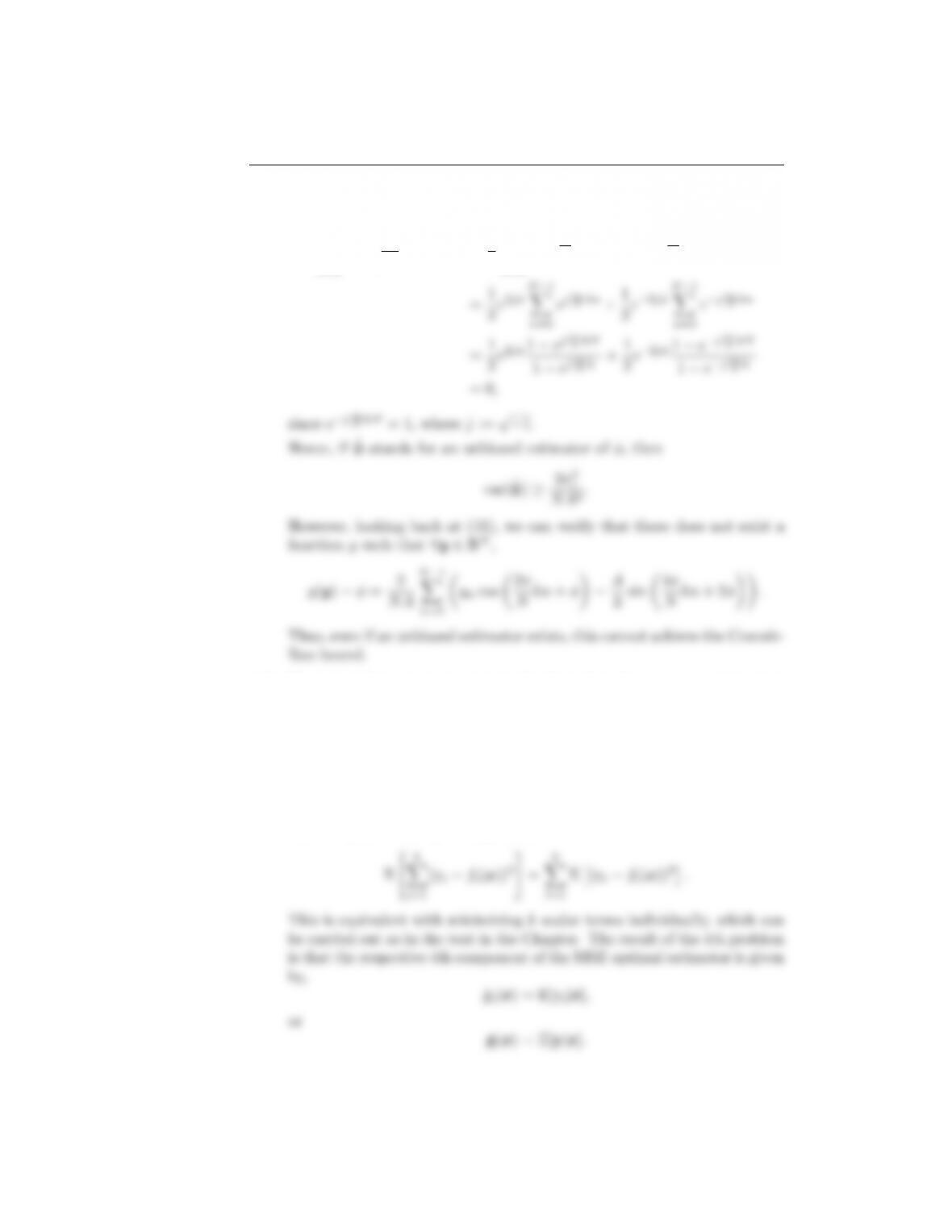
cos(2α))/2, and also the fact
N1
X
n=0
cos 4π
Nkn + 2φ=1
2
N1
X
n=0 ej(4π
Nkn+2φ)+ej(4π
Nkn+2φ)
N1
X
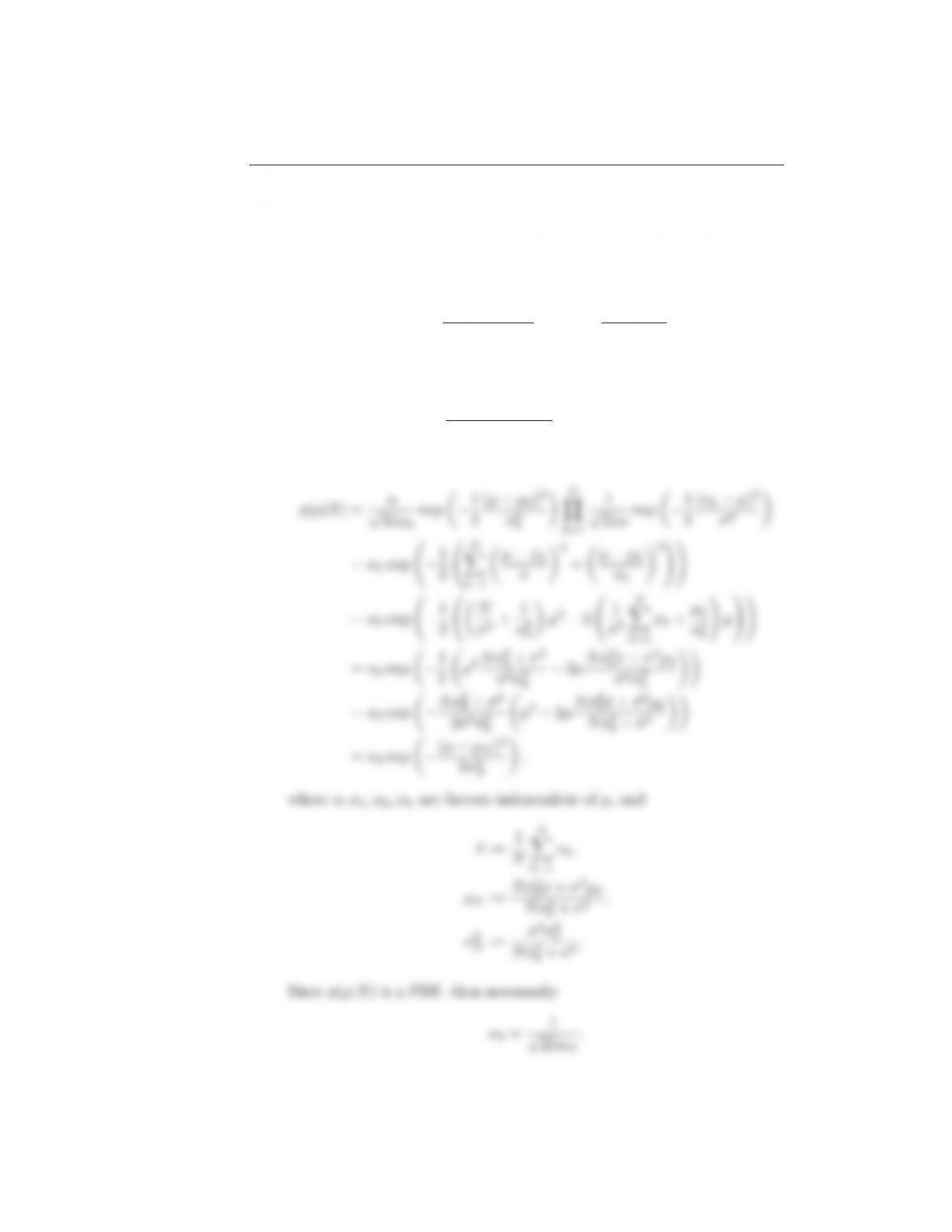
N1
X
3.15. Show that if (y,x) are two jointly distributed random vectors, with values
in Rk×Rl, then the MSE optimal estimator of ygiven the value x=x
is the regression of yconditioned on x, i.e., E[y|x].
Solution: The proof follows a similar line as the scalar case. Let
f(x) := [f1(x), . . . , fk(x)]T
be the vector estimator. Then the MSE optimal one should minimize the
sum of square errors per component, i.e.,
X
k
X
page-pf2
15
3.16. Assume that x,yare jointly Gaussian random vectors, with covariance
matrix
Σ:= Exµx
yµy(xµx)T,(yµy)T=ΣxΣxy
Σyx Σy.
Assuming also that the matrices Σxand ¯
Σ:= ΣyΣyxΣ1
xΣxy are
non-singular, then show that the optimal MSE estimator E[y|x] takes the
following form,
E[y|x] = E[y] + ΣyxΣ1
x(xE[x]).
Notice that E[y|x] is an affine function of x. In other words, for the case
where xand yare jointly Gaussian, the optimal estimator of y, in the
MSE sense, which is in general a non-linear function, becomes an affine
function of x.
In the special case where x,y are scalar random variables, then
E[y|x] = µy+ασy
σx
(xµx),
where αstands for the correlation coefficient, defined as
α:= E[(x µx)(y µy)]
σxσy
,
with |α| ≤ 1. Notice, also, that the previous assumption on the non-
singularity of Σxand ¯
Σtranslates, in this special case, to σx6= 0 6=σy,
and |α|<1.
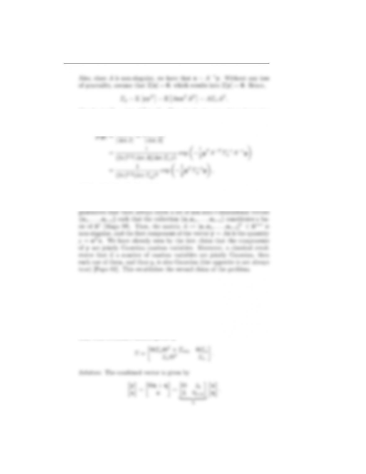
Solution: First, it is easy to verify that Σyx =ΣT
xy. Moreover, since
Σxand ¯
Σare assumed to be non-singular, then it can be verified, e.g.,
[Magn 99], that the determinant det Σ= det Σxdet ¯
Σ, and that
x+Σ1
xΣxy ¯
Σ1ΣyxΣ1
xΣ1
xΣxy ¯
Σ1
page-pf3
16
and ¯
y:= yµy. Then, the joint pdf of xand ybecomes
p(x,y) = 1
(2π)l(det Σ)1
2
exp 1
2¯
xT,¯
yTΣ1¯
x
¯
y
2¯
As a result, the marginal pdf p(x) becomes
p(x) = Zp(x,y)dy=1
(2π)l/2(det Σx)1
2
exp 1
2¯
xTΣ1
x¯
x
(2π)l/2(det Σx)1
2
2¯
Using the previous relations, we can easily see that
p(y|x) = p(x,y)
p(x)
yΣyxΣ1
x¯
xT¯
Σ1¯
yΣyxΣ1
x¯
x
3.17. Assume a number lof jointly Gaussian random variables {x1,x2,...,xl},
and a non-singular matrix ARl×l. If x:= [x1,x2,...,xl]T, then show
that the components of the vector y, obtained by y=Ax, are also jointly
Gaussian random variables.
A direct consequence of this result is that any linear combination of jointly
Gaussian variables is also Gaussian.
Solution: The Jacobian matrix of a linear transform y=Axis easily
shown to be
J:= J(y;x) = A.
page-pf4
17
Clearly, det Σy= (det A)2det Σx. Then, by the theorem of transformation
for random variables, e.g., [Papo 02], we have the following:
(2π)l/2(det Σy)1
2
2yTΣ1
which establishes the first claim.
For the second claim, assume a non-zero vector aRl, and define the lin-
ear combination of {x1,x2,...,xl}as y = aTx. Elementary linear algebra
3.18. Let xRlbe a vector of jointly Gaussian random variables, of covariance
matrix Σx. Consider the general linear regression model
y= Θx+η,
where Θ Rk×lis a parameter matrix and ηis the vector of noise samples,
which are considered to be Gaussian, with zero mean, and with covariance
matrix Ση, independent of x. Then show that yand xare jointly Gaus-
sian, with covariance matrix given by
|{z }
A
page-pf5
18
However, since xand ηare both Gaussian vector variables, and mutually
independent, then they are also jointly Gaussian. Notice also that the
3.19. Show that a linear combination of Gaussian independent variables is also
Gaussian.
Solution: This is a direct consequence of Problem 3.17, since independent
3.20. Show that if a sufficient statistic T(X) for a parameter estimation problem
exists, then T(X) suffices to express the respective ML estimate.
Solution: This is direct consequence of the Fisher-Neyman factorization
3.21. Show that if an efficient estimator exists then it is also optimal in the ML
sense.
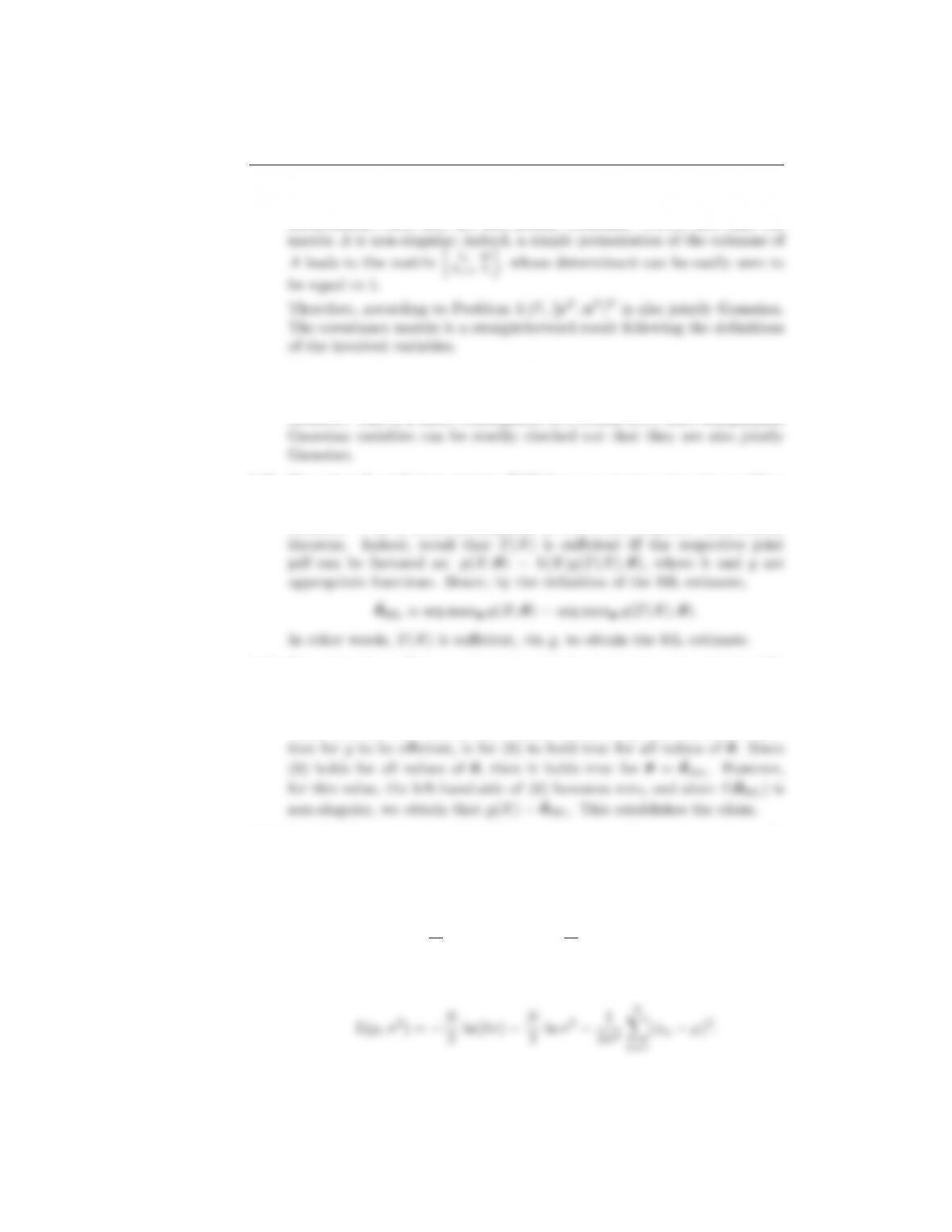
Solution: Assume the existence of an efficient estimator, i.e., a function g
which achieves the Cram´er-Rao bound. A necessary and sufficient condi-
3.22. Let the observations resulting from an experiment be xn,n= 1,2, . . . , N .
Assume that they are independent and that they originate from a Gaussian
PDF N(µ, σ2). Both, the mean and the variance, are unknown. Prove
that the ML estimates of these quantities are given by
ˆµML =1
N
N
X
n=1
xn,ˆσ2
ML =1
N
N
X
n=1
(xnˆµML)2.
Solution: The log-likelihood function is given by
2ln(2π)N
2ln σ21
2σ2
N
X
n=1
page-pf6
19
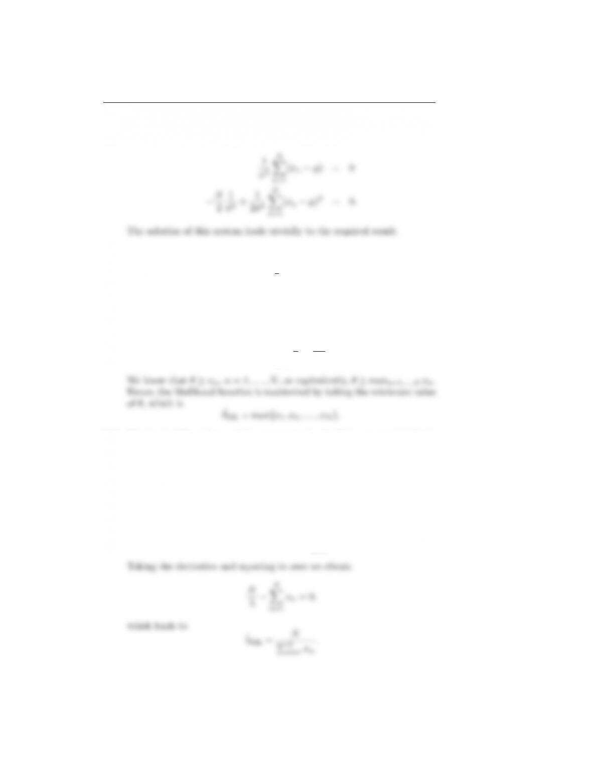
Taking the gradient with respect to µ, σ2, and equating it to zero we obtain
the following system of equations
N
X
3.23. Let the observations xn, n = 1,2, . . . , N, come from the uniform distribu-
tion
p(x;θ) = (1
θ,0< x θ,
0,otherwise.
Obtain the ML estimate of θ.
Solution: The likelihood function is given by
L(x;θ) =
N
Y
n=1
1
θ=1
θN.
3.24. Obtain the ML estimate of the parameter λ > 0 of the exponential distri-
bution
p(x) = (λexp(λx), x 0,
0, x < 0,
based on a set of measurements, xn,n= 1,2, . . . , N.
Solution: The log-likelihood function is
L(x;λ) = Nln λλ
N
X
n=1
xn.
n=1 xn
page-pf7
20
3.25. Assume an µ∼ N(µ0, σ2
0), and a stochastic process {xn}
n=−∞, consisting
of i.i.d random variables, such that p(xn|µ) = N(µ, σ2). Consider N
observations so that X ≡ {x1, x2, . . . , xN}, and prove that the posterior
p(x|X), of any x=xn0conditioned on X, turns out to be Gaussian with
mean µNand variance σ2+σ2
N, where
µNNσ2
0¯x+σ2µ0
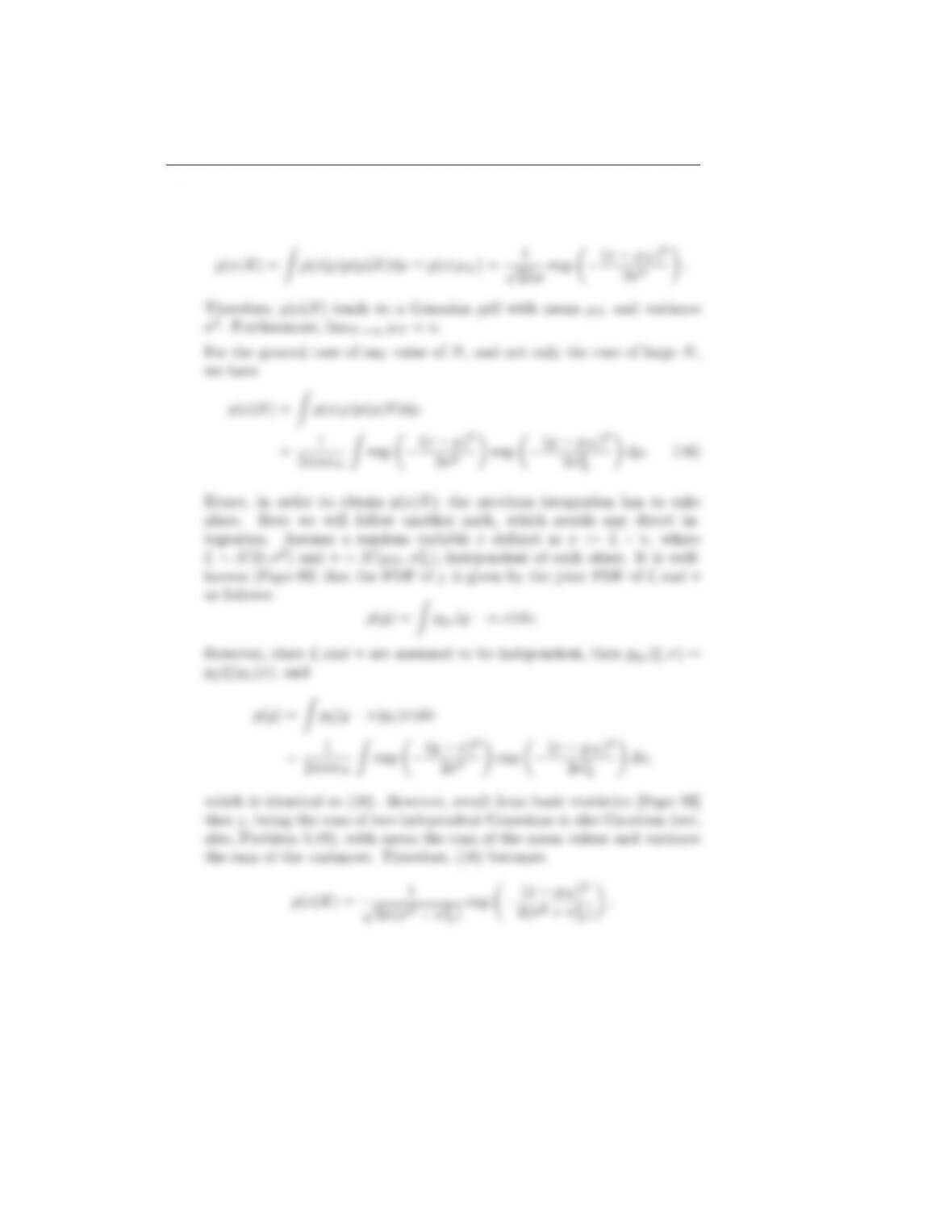
Nσ2
0+σ2, σ2
Nσ2σ2
0
Nσ2
0+σ2.
Solution: From basic theory we have that
p(µ|X) = p(X|µ)p(µ)
Rp(X|µ)p(µ)=αp(µ)
N
Y
k=1
p(xk|µ),
or
(µµ0)2
Y
1
(xkµ)2
page-pf8
21
Hence, limN→∞ σ2
N= 0, and for large N,p(µ|X) behaves like a δfunction
centered around µN. Thus,
3.26. Show that for the linear regression model,
y=Xθ+η,
the a-posteriori probability p(θ|y) is a Gaussian one, if the prior distri-
bution probability is given by p(θ) = N(θ, Σ0), and the noise samples
page-pf9
22
follow the multivariate Gaussian distribution p(η) = N(0, Ση). Compute
the mean vector and the covariance matrix of the posterior distribution.
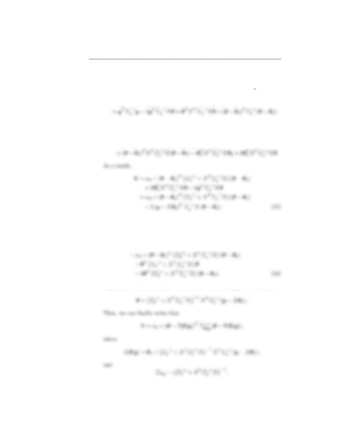
Solution: It can be easily checked that p(θ|y) = const×exp 1
2Ψ, where
Ψ = (yXθ)TΣ1
η(yXθ) + (θθ0)TΣ1
0(θθ0)
From now on, all terms that will be independent of θwill be collected in
constant terms. Hence
Ψ = α12yTΣ1
ηXθ+ (θθ0)TΣ1
0(θθ0)
In the sequel, we will follow a standard trick that we do in situations
like that. We introduce an auxiliary variable ¯
θ, whose value is to be
determined so that to make the following to be true,
Ψ = α4+ (θθ0¯
θ)TΣ1
0+XTΣ1
ηX(θθ0¯
θ)
Inspection of (17) and (18) indicates that this can happen if we choose
page-pfa
23
3.27. Assume that xn,n= 1,2...,N, are i.i.d observations from a Gaussian
N(µ, σ2). Obtain the MAP estimate of µ, if the prior follows the expo-
nential distribution
p(µ) = λexp (λµ), λ > 0, µ 0.
Solution: Upon defining X:= {x1, x2, . . . , xN}, the posterior distribution
is given by
p(µ|X)p(X|µ)p(µ) = λexp (λµ)
(2π)N/2σN
N
Y
n=1
exp (xnµ)2
2σ2.
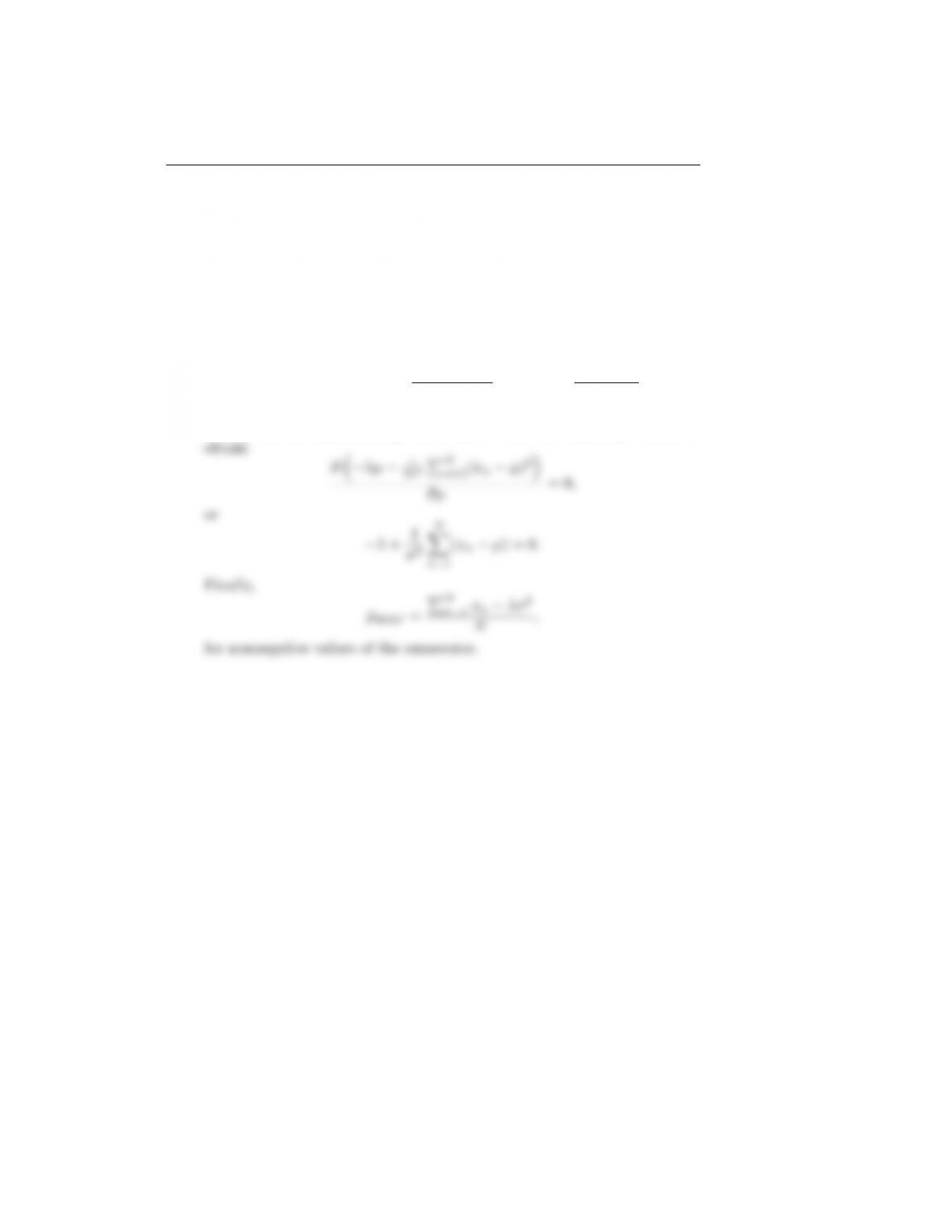
Taking the ln, differentiating with respect to µ, and equating to zero we
24
page-pfc
Bibliography
[Magn 99] Magnus, J. R., and Neudecker, H. Matrix Differential Calculus with
Applications in Statistics and Econometrics. John Wiley & Sons,
revised Ed., 1999.
25

Trusted by Thousands of
Students

Here are what students say about us.

Copyright ©2022 All rights reserved. | CoursePaper is not sponsored or endorsed by any college or university.