Unlock document.
This document is partially blurred.
Unlock all pages and 1 million more documents.
Get Access

1
Solutions To Problems of Chapter 2
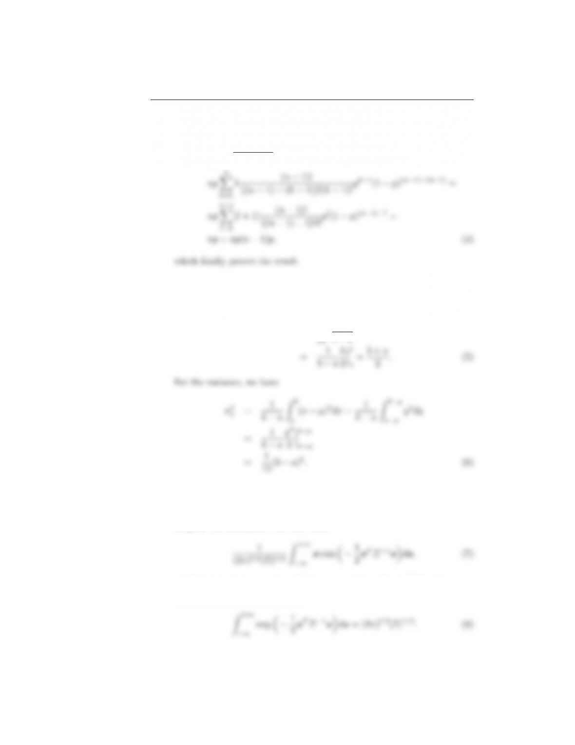
2.1. Derive the mean and variance for the binomial distribution.
Solution: For the mean value we have that,
E[x] =
n
X
k=0
kn!
(n−k)!k!pk(1 −p)n−k
n
X
n!
where the formula for the binomial expansion has been employed. For the
variance we have,
σ2
x=
n
X
k=0
(k−np)2n!
(n−k)!k!pk(1 −p)n−k
n
X
k=0
2
However,
n
X
k=0
k2n!
(n−k)!k!pk(1 −p)n−k=
n
X
2.2. Derive the mean and the variance for the uniform distribution.
Solution: For the mean we have
µ=E[x] = Zb
1
b
b
2.3. Derive the mean and covariance matrix of the multivariate Gaussian.
Solution: Without harming generality, we assume that µ=0, in order to
simplify the discussion. We have that
which due to the symmetry of the exponential results in E[x] = 0.
For the covariance we have that
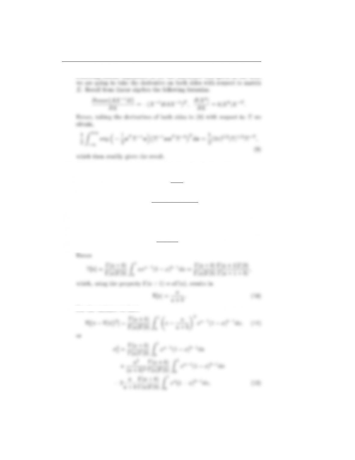
3
Following similar arguments as for the univariate case given in the text,
2.4. Show that the mean and variance of the beta distribution with parameters
aand bare given by
E[x] = a
a+b,
and
σ2
x=ab
(a+b)2(a+b+ 1).
Hint: Use the property Γ(a+ 1) = aΓ(a).
Solution: We know that
Beta(x|a, b) = Γ(a+b)
Γ(a)Γ(b)xa−1(1 −x)b−1.
For the variance we have
a+b
Γ(a)Γ(b)Z1
0
4
2.5. Show that the normalizing constant in the beta distribution with param-
eters a, b is given by
Γ(a+b)
Γ(a)Γ(b).
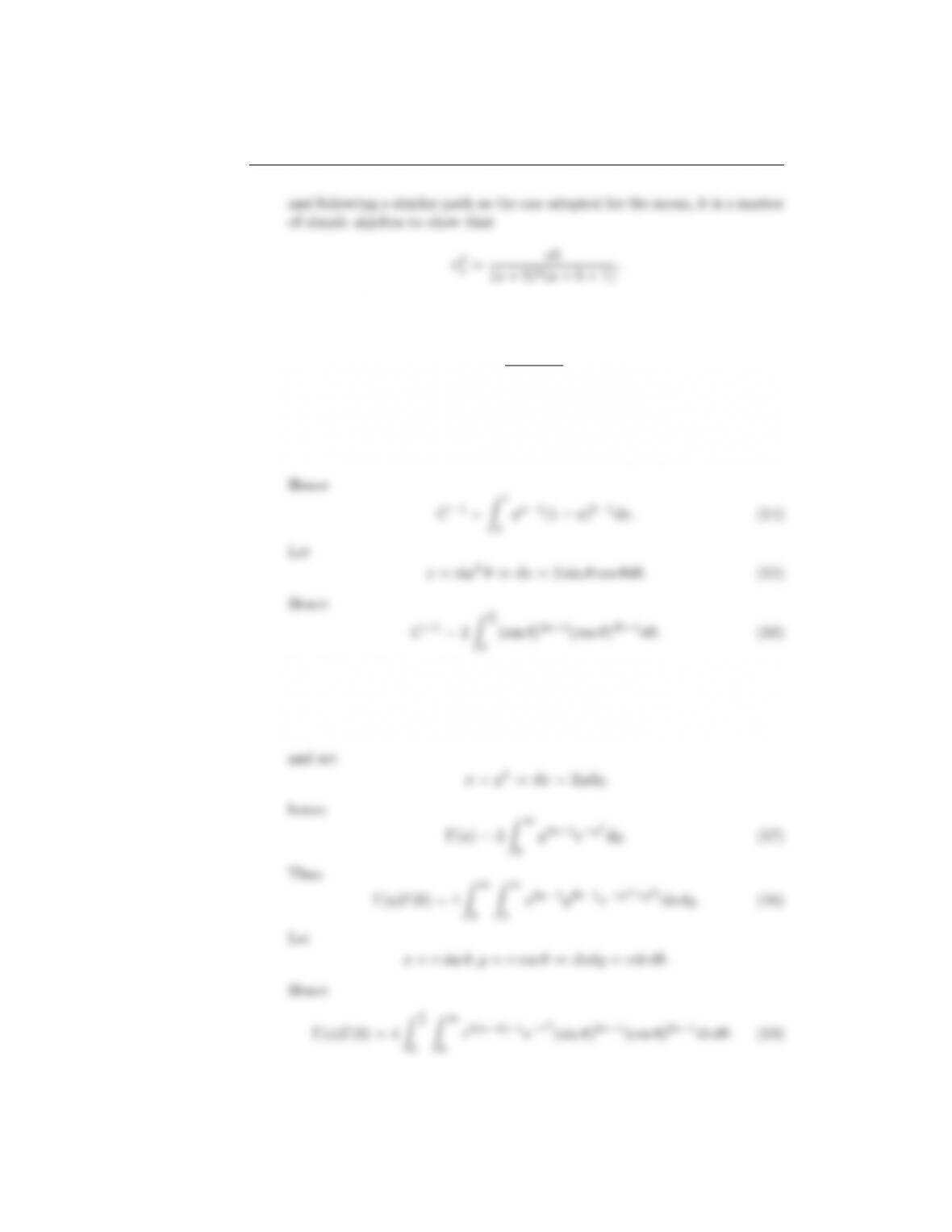
Solution: The beta distribution is given by
Beta(x|a, b) = Cxa−1(1 −x)b−1,0≤x≤1.(13)
0
Recall the definition of the gamma function
Γ(a) = Z∞
0
xa−1e−xdx,
0Z∞
0
5
2.6. Show that the mean and variance of the gamma pdf
Gamma(x|a, b) = ba
Γ(a)xa−1e−bx, a, b, x > 0.
are given by
E[x] = a
b,
σ2
x=a
b2.
Solution: We have that
E[x] = ba
Γ(a)Z∞
0
xae−bxdx.
Set bx =y. Then
E[x] = ba
Γ(a)
1
ba+1 Z∞
0
yae−ydy
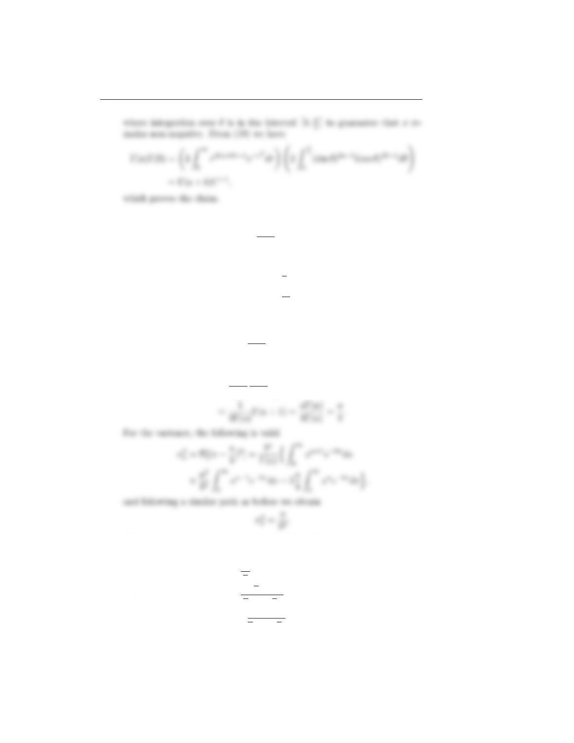
2.7. Show that the mean and variance of a Dirichlet pdf with Kvariables,
xk, k = 1,2, . . . , K and parameters ak, k = 1,2, . . . , K, are given by
E[xk] = ak
a, k = 1,2, . . . , K
σ2
k=ak(a−ak)
a2(1 + a), k = 1,2, . . . , K,
cov[xixj] = −aiaj
a2(1 + a), i 6=j,
6
where a=PK
k=1 ak.
Solution: Without harm of generality, we will derive the mean for xK.
The others are derived similarly. To this end, we have
p(x1, x2, . . . , xK−1) = C
K−1
Y
k=1
xak−1
k 1−
K−1
X
k=1
xk!aK−1
where
E[xK] = CZ1
0
· · · Z1
0
K−1
Y
xak−1
k 1−
K−1
X
xk!aK
dxK−1. . . dx1
7
be taken in place of xKand xK−1. Hence,
E[xK−1xK] = CZ1
0
· · · Z1
0"Z1−PK−1
k=1 xk
0 K−2
Y
k=1
xak−1
k!xaK−1
K−1xaK
KdxK#dxK−1. . . dx1
K−2
Y
k=1 xk
or
E[xK−1xK] = aKaK−1
a(1 + a).
2.8. Show that the sample mean, using Ni.i.d drawn samples, is an unbiased
estimator with variance that tends to zero asymptotically, as N−→ ∞.
Solution: From the definition of the sample mean we have
E[ˆ
µN] = 1
N
N
X
n=1
E[xn] = 1
N
N
X
n=1
E[x] = E[x].(20)
8
For the variance we have,
σ2
ˆµN=E
1
N
N
X
i=1
xi−µ!
1
N
N
X
j=1
xj−µ
1
N
X
N
X
2.9. Show that for WSS processes
r(0) ≥ |r(k)|,∀k∈Z,
and that for jointly WSS processes,
ru(0)rv(0) ≥ |ruv(k)|2,∀k∈Z.
Solution: Both properties are shown in a similar way. So, we are going to
focus on the first one. Consider the obvious inequality,
E[|un−λun−k|2]≥0,
or
E[|un|2] + |λ|2E[|un−k|2]≥λ∗r(k) + λr∗(k),
9
2.10. Show that the autocorrelation of the output of a linear system, with im-
pulse response, wn, n ∈Z, is related to the autocorrelation of the input
process, via,
rd(k) = ru(k)∗wk∗w∗
−k.
Solution: We have that
rd(k) = E[dnd∗
n−k] = E
X
i
w∗
iun−iX
j
wju∗
n−k−j
2.11. Show that
ln x≤x−1.
Solution: Define the function
f(x) = x−1−ln x.
2.12. Show that
I(x; y) ≥0.
10
Hint: Use the inequality of Problem 2.11.
Solution: By the respective definition, we have that
−I(x; y) = −X
xX
y
P(x, y) log P(x|y)
P(x)
2.13. Show that if ai, bi, i = 1,2, . . . , M are positive numbers, such as
M
X
i=1
ai= 1,and
M
X
i=1
bi≤1,
then
−
M
X
i=1
ailn ai≤ −
M
X
i=1
ailn bi.
Solution: Recalling the inequality from Problem 2.11, that
ln bi
ai
≤bi
ai
−1,
2.14. Show that the maximum value of the entropy of a random variable occurs
if all possible outcomes are equiprobable.
11
Solution: Let pi, i = 1,2, . . . , M, be the corresponding probabilities of
the Mpossible events. According to the inequality in Problem 2.13 for
2.15. Show that from all the pdfs which describe a random variable in an inter-
val [a, b] the uniform one maximizes the entropy.
Solution: The Lagrangian of the constrained optimization task is
L(p(·), λ) = −Z+∞
−∞
p(x) ln p(x)dx +λZ+∞
−∞
p(x)dx −1.


