Machine Learning Chapter 18 Solutions Problems Prove That The Perceptron Algorithm Its Patternbypattern Mode Operation

subject Type Homework Help
subject Pages 9
subject Words 2654
subject Authors Sergios Theodoridis

Unlock document.

This document is partially blurred.
Unlock all pages and 1 million more documents.
Get Access
page-pf1
1
Solutions To Problems of Chapter 18
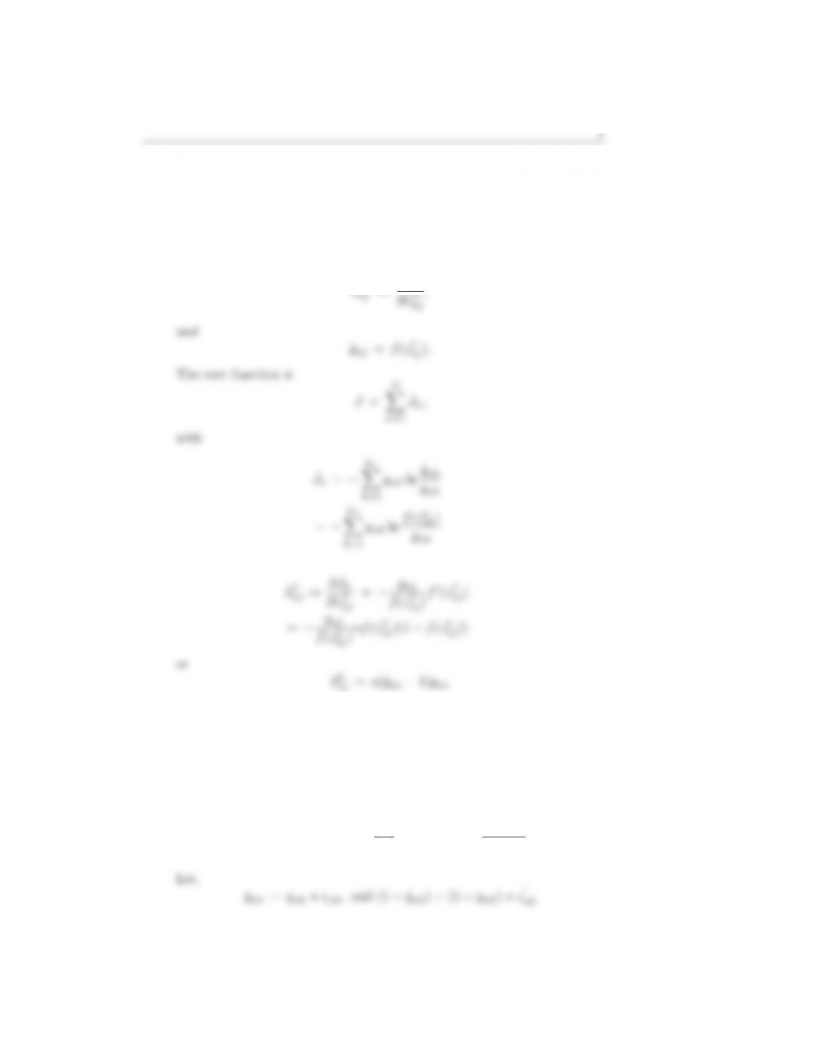
18.1. Prove that the perceptron algorithm, in its pattern-by-pattern mode of
operation, converges in a finite number of iteration steps. Assume that
θ(0) =0.
Hint: Note that since classes are assumed to be linearly separable, there
exists a normalized hyperplane, θ, and a γ > 0, so that
γynθT
xn, n = 1,2, . . . , N,
where, ynis the respective label, being +1 for ω1and 1 for ω2. By the
term normalized hyperplane, we mean that,
θT
= [ ˆ
θ, θ0]T,with ||ˆ
θ|| = 1.
In this case, ynθT
xnis the distance of xnfrom the hyperplane θ([164]).
Solution: Let us assume that we are currently at iteration i. This means
that so far i1 update corrections have been performed by the algo-
rithm. The ith update will be performed only if the current sample, x(i),
is misclassified, i.e., only if
y(i)xT
(i)θ(i1) 0,
and the update will be
Also from (1), we have that
||θ(i)||2=||θ(i1)||2+ 2µy(i)xT
(i)θ(i1) + (4)
µ2y2
(i)||x(i)||2
page-pf2
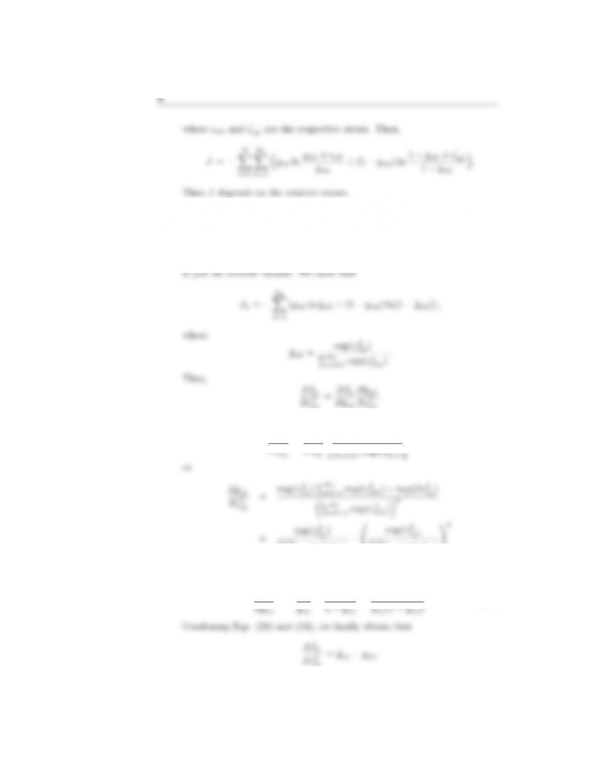
18.2. The derivative of the sigmoid functions has been computed in Problem
7.6. Compute the derivative of the hyperbolic tangent activation function
and show that it is equal to,
f0(z) = ac1f2(z).
Solution: We have that,
f(z) = atanh(cz)f0(z) = (ac) cosh2cz)
or
18.3. Show that the effect of the momentum term in the gradient descent back-
propagation scheme is to effectively increase the learning convergence rate
of the algorithm.
Hint: Assume that the gradient is approximately constant over Isucces-
sive iterations.
Solution Let idenote the current iteration, i.e.,
θr
j(i) = aθr
j(i1) µg,(8)
page-pf3
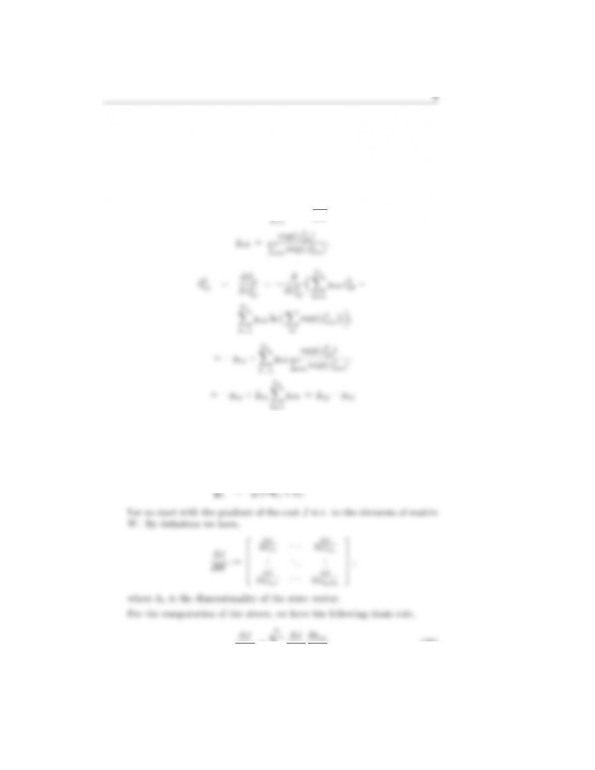
18.4. Show that if a) the activation function is the hyperbolic tangent, b) the
input variables are normalized to zero mean and unit variance, then in
order to guarantee that all the outputs of the neurons are zero mean and
unit variance, the weights must be drawn from a distribution of zero mean
and standard deviation equal to
σ=m1/2,
where mis the number of synaptic weights associated with the correspond-
ing neuron.
Hint: For simplicity, consider the bias to be zero, and also that the inputs
to each neuron are mutually uncorrelated.
Solution: Let us focus on the weights of a specific neuron, and denote
by yi, i = 1,2, . . . , m, the respective inputs. Then, the input to the acti-
vation functions will be given by
m
X
i=1
Assume that the inputs to the neuron are zero mean and unit variance
and are also uncorrelated, then
σ2
i=E[y2
i] (12)
and
E[yiyj] = δij .(13)
page-pf4
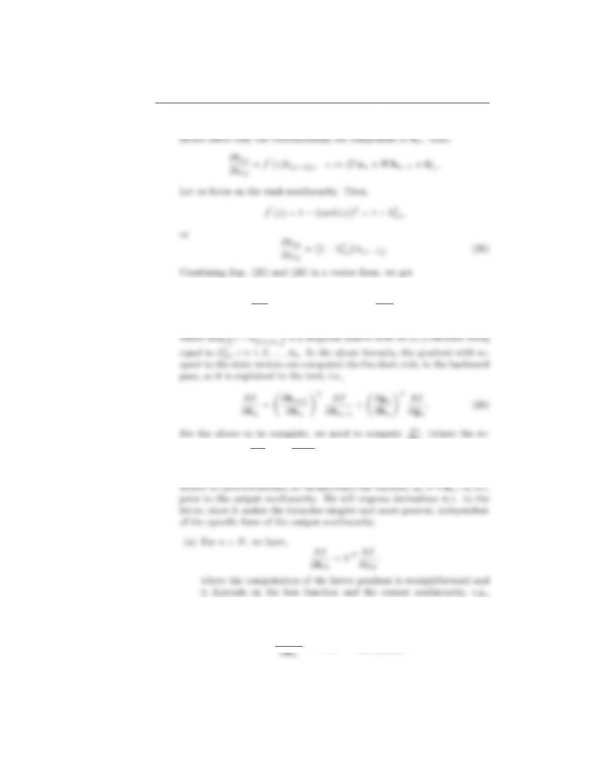
18.5. Consider the sum of error squares cost function
J=1
2
N
X
n=1
kL
X
m=1
(ˆynm ynm)2.(15)
Compute the elements of the Hessian matrix
2J
θr
kj θr0
k0j0
.(16)
Near the optimum, show that the second order derivatives can be approx-
imated by
2J
θr
kj θr0
k0j0
=
N
X
n=1
kL
X
m=1
ˆynm
θr
kj
ˆynm
θr0
k0j0
.(17)
In other words, the second order derivatives can be approximated as prod-
ucts of the first order derivatives. The derivatives can be computed by fol-
lowing similar arguments as the gradient descent backpropagation scheme,
[71].
Solution:
J=1
2
N
X
n=1
kL
X
m=1
(ˆynm ynm)2
J
θr
kj
=
N
X
n=1
kL
X
m=1
ˆynm
θr
kj
(ˆynm ynm)
2J
θr0
=
N
X
kL
X
2ˆynm
θr0
(ˆynm ynm)
N
X
kL
X
ˆynm
ˆynm
18.6. It is common when computing the Hessian matrix, to assume that it is
diagonal. Show, that under this assumption, the quantities
2E
(θkj )2,
where
kL
X
page-pf5
L)2=f00 (zL
2E
(zr1
k)2= (f0(zr1
j))2Pk2E
(zr
k)2(θr
kj )2+f00 (zr1
j)Pkr
k=1 θr
klδr
k.
(θr
kj )2=2E
(zr
j)2(yr1
k)2.(20)
For the backpropagation of the involved second derivatives, we have
I:r=L:E
=f0(zL
j)ej
We know from the text that,
δr1
j=
kr
X
δr
k
zr
k
zr1
=
kr
X
δr
kθr
kj f0(zr1
j) (21)
k=1
zr1
j
or
2E
(zr1
j)
kl
X
θr
kj δr
k+
kl
X
θr
kj
δr
k
zr1
f0(zr1
j) (22)
page-pf6
(zr
k)2θr
Thus, finally we get,
2E
2E
kr
X
18.7. Show that if the activation function is the logistic sigmoid and the loss
function in (18.44) is used, then δL
nj in (18.21) becomes
δL
nj =a(ˆynj ynj ).
If the cross-entropy in Eq. (18.41) is used, then it is equal to
δL
nj =aynj (ˆynj 1).
Solution: The cost function is
J=
N
X
n=1
Jn,
page-pf7
18.8. Show that if the activation function is the logistic sigmoid and the relative
entropy loss function is used, then δL
nj in (18.21) becomes,
δL
nj =a(ˆynj 1)ynj .
Solution: From the theory, we have that
18.9. Show that the cross-entropy loss function depends on the relative output
errors.
Solution: We will prove it for one of the versions, and similar is the proof
for the other. Taking into consideration the limiting value 0 ln 0 = 0, we
can write the cross-entropy cost as,
J=
N
X
n=1
kL
X
k=1 ynk ln ˆynk
ynk
+ (1 ynk) ln 1ˆynk
1ynk .
page-pf8
18.10. Show that if the activation function is the softmax and the loss function
is the cross-entropy (or the loss in (18.44)), then δL
nj in (18.21) does not
depend on the derivatives of the nonlinearity.
Solution: We will show it for Eq. (18.44) and for the cross-entropy it
nj
nj
Now,
ˆynj
zL
=
zL
nj )
PkL
m=1 exp(zL
nm) exp(zL
m=1 exp(zL
nm)!2
= ˆynj (1 ˆynj ).(23)
Also,
Jn
=ynj
+1ynj
=ˆynj ynj
nj
page-pf9
18.11. As in the previous problem, use the relative entropy as the cost function
and the softmax activation function. Then show that,
δL
nj = ˆynj ynj .
Solution:
Jn=
kL
X
ynk ln ˆynk
ynk
,
nk)
k=1
18.12. Derive the backpropagation through time algorithm for training recurrent
neural networks.
Solutions: The starting set of equations are those defining an RNN, i.e.,
hn=f(Uxn+Whn1+b),
wij
=
n=1
hni
wij
.(25)
page-pfa
10
Note from the defining RNN equations, all the wij ,j= 1,2, . . . , kh, ele-
J
W =
N
X
n=1
diag 1h2
ni:1,khJ
hn
hT
n1,(27)
hN(where the re-
cursion starts), ˆ
yn
hnand hn+1
hn. The gradient of the cost w.r. to the
outputs is straightforward, and depends on the specific loss function, see,
e.g., Problem 18.10.
Problem 18.10.
(b) Also, following similar arguments as before,
hn+1
= diag(1 h2
(n+1)i:1,kh)W.
page-pfb
is straightforward.
The above have completed the calculations of the gradient of Jw.r. to
W.
For the gradient w.r. to V, we get,
J
V =
N
X
J
zn
hT
n
c=
n=1 zn
cTJ
zn
=
n=1
zn
The gradient w.r. to bis equal to,
J
b=
N
X
bTJ
hn
N
X
18.13. Derive the gradient of the log-likelihood in (18.74).
Solutions: To simplify slightly the notation, we will consider only one
term of the sum. Thus we have,
P (v; Θ)
=
ln X
exp (E)(29)
θij
vX
h
page-pfc
18.14. Prove that for the case of RBMs, the conditional probabilities are given
by the following factorized form,
P(h|v) =
I
Y
exp PJ
j=1 θij vj+bihi
page-pfd
18.15. Derive Eq. (18.83).
Solution: The integrand is equal to

Trusted by Thousands of
Students

Here are what students say about us.

Copyright ©2022 All rights reserved. | CoursePaper is not sponsored or endorsed by any college or university.