Machine Learning Chapter 14 Solutions Problems Show That Fxx The Cumulative Distribution Function Random Variable

subject Type Homework Help
subject Pages 9
subject Words 1966
subject Authors Sergios Theodoridis

Unlock document.

This document is partially blurred.
Unlock all pages and 1 million more documents.
Get Access
page-pf1
1
Solutions To Problems of Chapter 14
14.1. Show that if Fx(x) is the cumulative distribution function of a random
variable x, then the random variable u = Fx(x) follows the uniform distri-
bution in [0,1].
Solution: Let
u = Fx(x),0u1.
Then, we have that
14.2. Show that if u follows the uniform distribution and
x = F1
x(u) := g(u),(1)
then indeed x is distributed according to Fx(x) = Rx
−∞ p(x)dx.
Solution: Due to the monotonicity of Fx(x), for each xthere exists a
unique u. Let ˜p(x) be the pdf of the generated x by (1). We have that
x = F1
x(u) or
0
14.3. Consider the random variables r and φwith exponential and uniform
distributions
pr(r) = 1
2exp r
2, r 0
and
pφ(φ) = 1
2π0φ2π
0 otherwise,
page-pf2
2
respectively. Show that the transformation
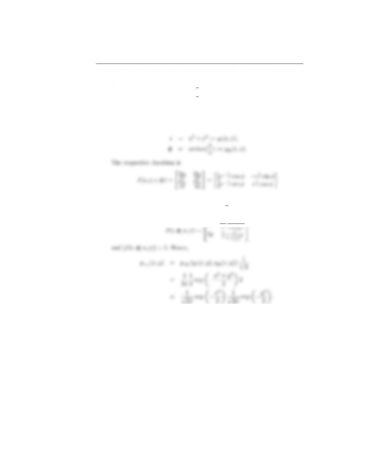
x = r cos φ=gx(r,φ),
y = r sin φ=gy(r,φ),
renders both x and y to follow the normalized Gaussian N(0,1).
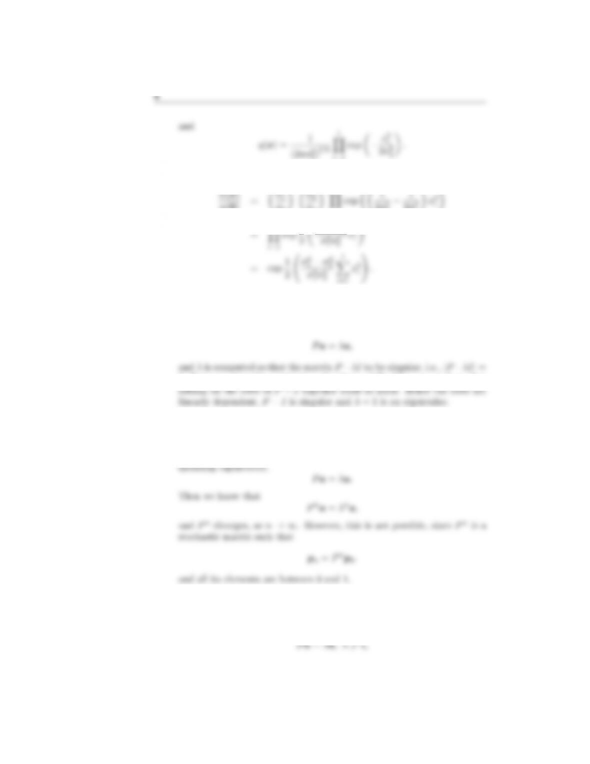
Solution: We have that
r
φ #=1
2r1
and
|J(x,y; r,φ)|=1
2.
Note that
2xy
1
14.4. Show that if
px(x) = N(x|0, I),
then ygiven by the transformation
y=Lx+µ
is distributed according to
py(y) = N(y|µ, Σ),
where Σ=LLT.
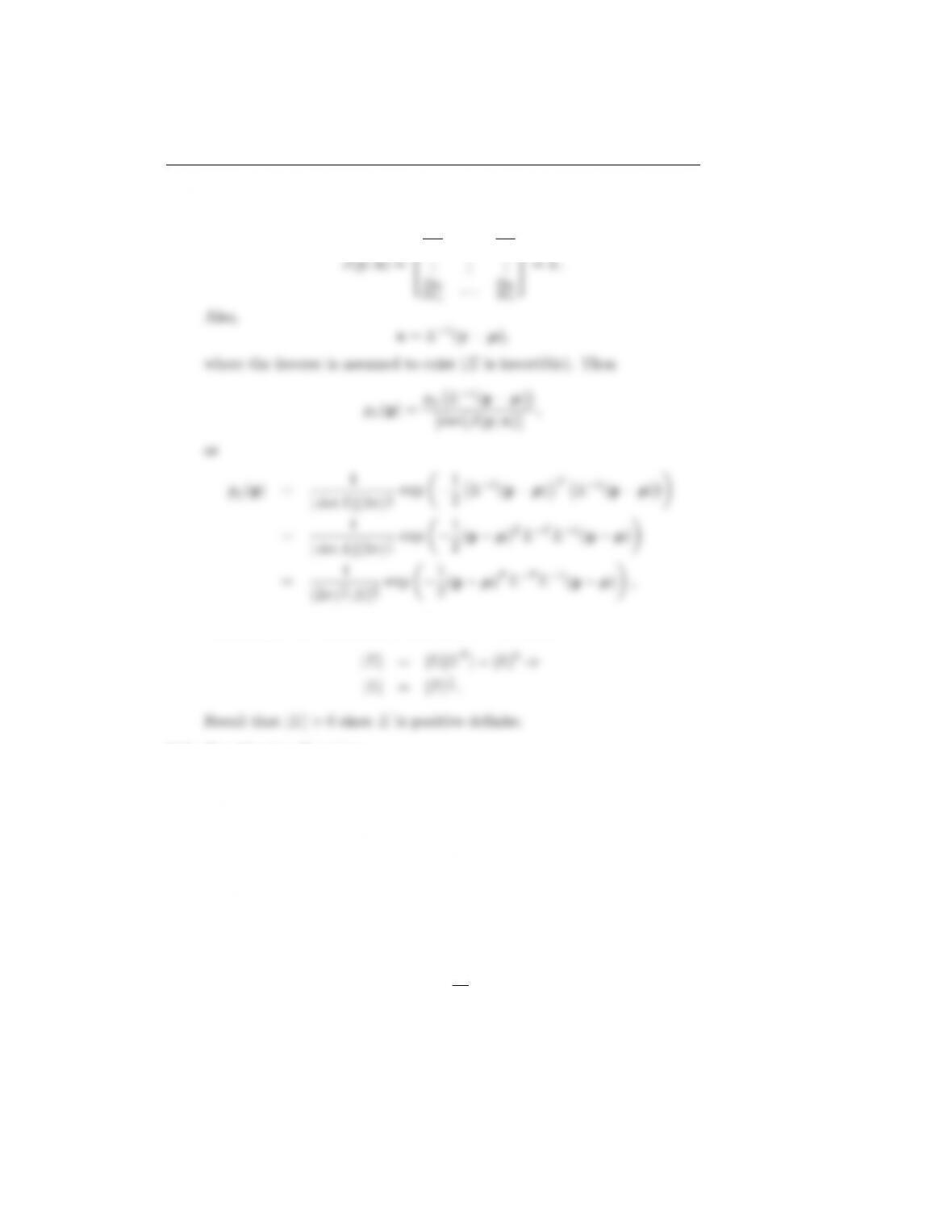
Solution: We have that,
y=Lx+µ,
page-pf3
3
is a linear transformation and it is readily checked out that the Jacobian
matrix
y1
x1. . . y1
xl
.
where |Σ|is the determinant of Σand we used that
14.5. Consider two Gaussians
p(x) = N(x|0, σ2
pI), σ2
p= 0.1
and
q(x) = N(x|0, σ2
qI), σ2
q= 0.11
xRl. In order to use q(x) for drawing samples from p(x), via the
rejection sampling method, a constant chas to be computed so that
cq(x)p(x).
Show that
cσq
σpl
,
and compute the probability of accepting samples.
page-pf4
4
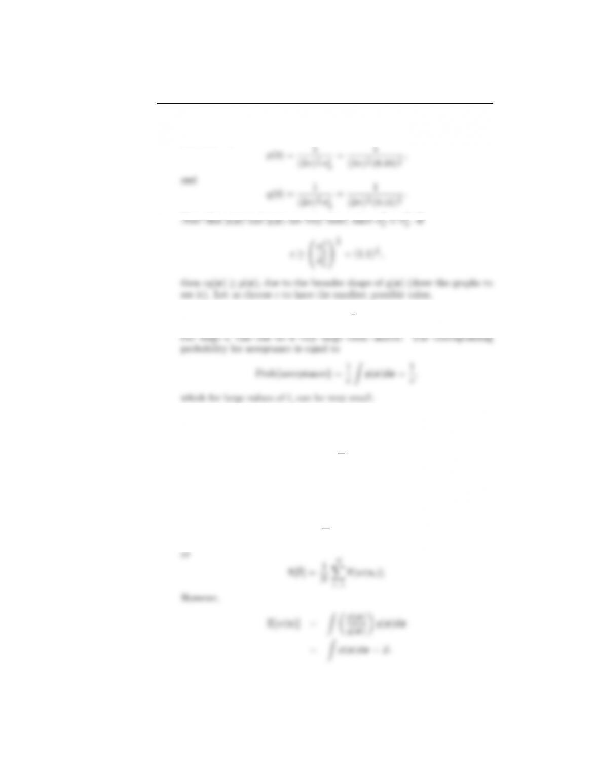
Solution: The maximum values for the two distributions occur at x= 0
and they are
c= (1.1) l
2.
14.6. Show that using importance sampling leads to an unbiased estimator for
the normalizing constant of the desired distribution,
p(x) = 1
Zφ(x).
However, the estimator E[f(x)], of a function f(·) is a biased one.
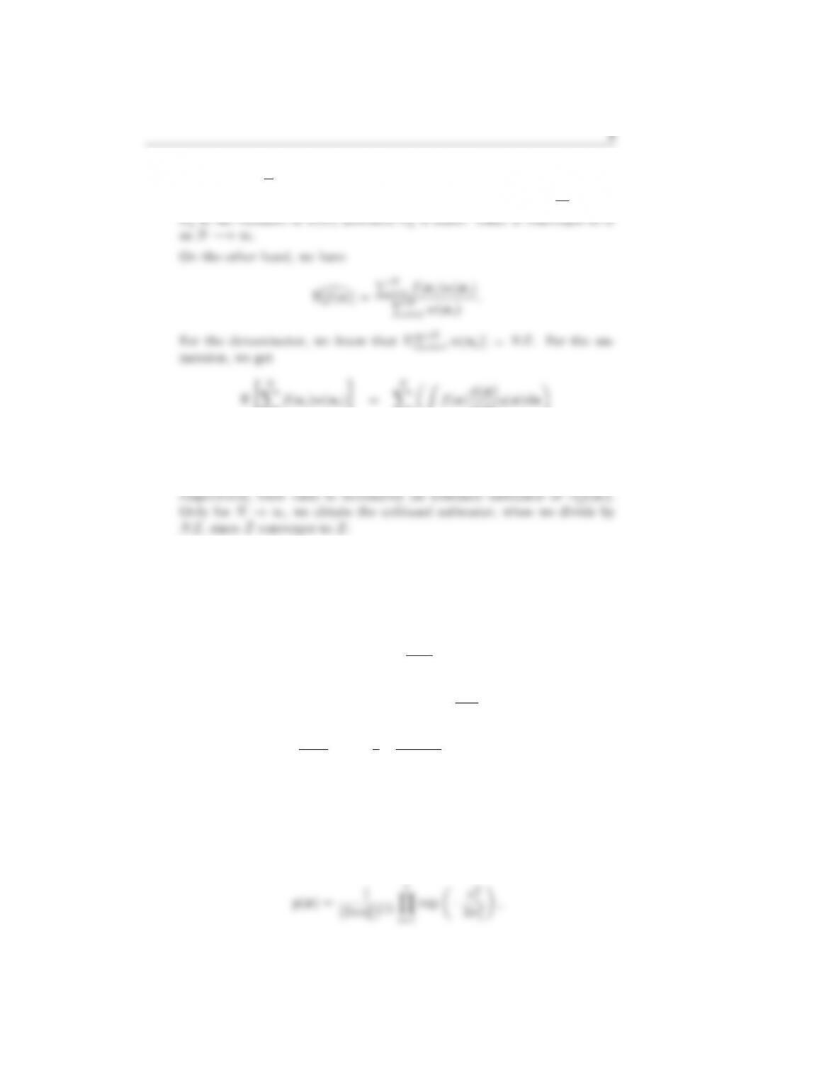
Solution: We know that
ˆ
Z=1
N
N
X
i=1
w(xi)
page-pf5
Hence E[ˆ
Z] = 1
NNZ =Z. Also, since ˆ
Z is the sum of Nunbiased variables
divided by N, we know (Chapter 3) that its variance will be σ2
w
N, where
E"N
i=1
f(xi)w(xi)#=
i=1 Zf(x)φ(x)
q(x)q(x)dx
=NZ ·E[f(x)]
However, for finite number of N, this does not mean that although the
mean values of the numerator and denominator are NZ ·E[f(x)] and NZ,
14.7. Let p(x) = N(x|0, σ2
1I). Choose the proposal distribution for importance
sampling as
q(x) = N(x|0, σ2
2I).
The weights are computed as
w(x) = p(x)
q(x).
If w(0) is the weight at x=0, then the ratio w(x)
w(0)is given by
w(x)
w(0)= exp 1
2 σ2
1σ2
2
σ2
1σ2
2
l
X
i=1
x2
i!.
Observe that even for very good match between q(x) and p(x) (σ2
1'σ2
2),
for large values of l, the values of the weights can change significantly, due
to the exponential dependence.
Solution: We have that
l
Y
i
page-pf6
2)l/2
Hence,
Y
2 σ2
σ2
1σ2
2
i=1
14.8. Show a stochastic matrix Phas always the value λ= 1 as its eigenvalue.
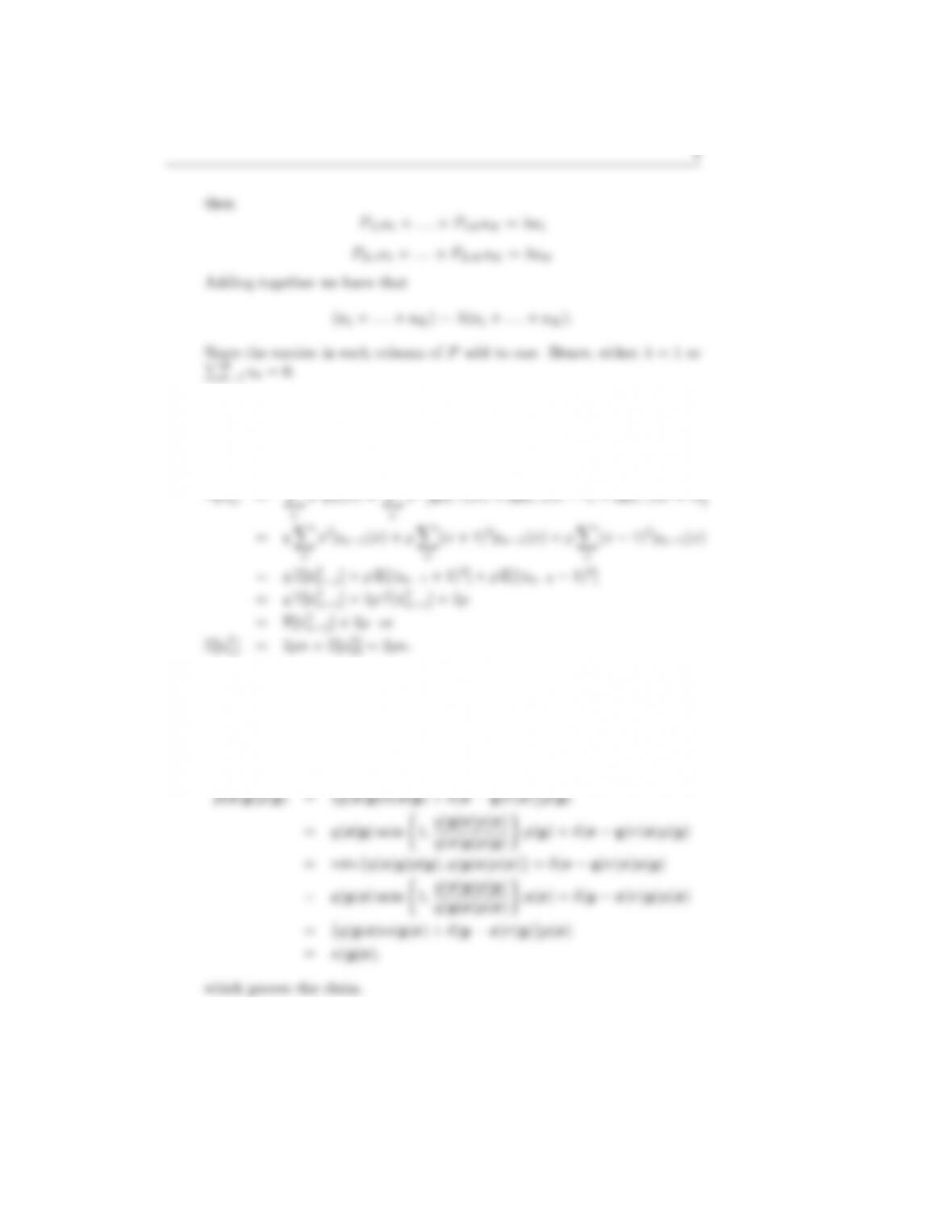
Solution: By definition we have
0. However, since the entries in each column of Padd to one we have that
14.9. Show that if the eigenvalue of a transition matrix is not equal to one, its
magnitude can not be larger than one, i.e., |λ| ≤ 1.
Solution: Let λbe an eigenvalue such that |λ|>1, with aits corre-
14.10. Prove that if Pis a stochastic matrix and λ6= 1, then the elements of the
corresponding eigenvector add to zero.
Solution: Let
page-pf7
14.11. Prove the square root dependence of the distance travelled by a random
walk, with infinite many integer states, on the time, n.
Solution: We have that
14.12. Prove, using the detailed balance condition, that the invariant distribu-
tion associated with the Markov chain implied by the Metropolis-Hastings
algorithm is the desired distribution, p(x).
Solution: By the definition of the respective kernel density we have
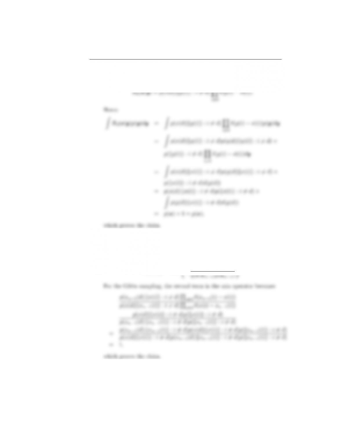
14.13. Show that in Gibbs sampling, the desired joint distribution is invariant
with respect to each one of the base transition pdfs.
page-pf8
8
Solution: By the definition of the base transition pdfs we have
14.14. Show that the acceptance rate for the Gibbs sampling is equal to one.
Solution: We know that the acceptance ratio for the Metropolis-Hastings
algorithm is given by
α(x|xn) = min 1,q(xn1|x)p(x)
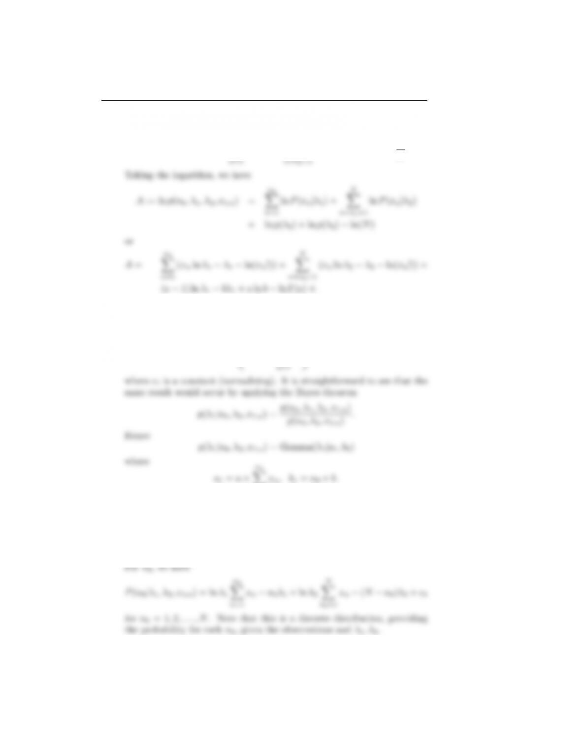
14.15. Derive the formulae for the conditional distributions of Section 14.11
page-pf9
9
Solution: The joint distribution of n0, λ1, λ2, x1:Nis given by
p(n0, λ1, λ2, x1:N) =
n0
Y
P(xn|λ1)
N
Y
P(xn|λ2)p(λ1)p(λ2)1
N.
(a1) ln λ22+aln bln Γ(a)ln N.
To get the conditionals, it suffices to freeze the values of the rest of vari-
ables and consider them constants. For example,
ln p(λ1|n0, λ2, x1:n) = a1 +
n0
X
xn!ln λ1(n0+b)λ1+c1,
n=1
Similarly
p(λ2|n0, λ1, x1:n) = Gamma(λ2|a2, b2)
a2=a+
N
X
n=n0+1
xn, b2=Nn0+b.

Trusted by Thousands of
Students

Here are what students say about us.

Copyright ©2022 All rights reserved. | CoursePaper is not sponsored or endorsed by any college or university.