Unlock document.
This document is partially blurred.
Unlock all pages and 1 million more documents.
Get Access
1
Solutions To Problems of Chapter 12
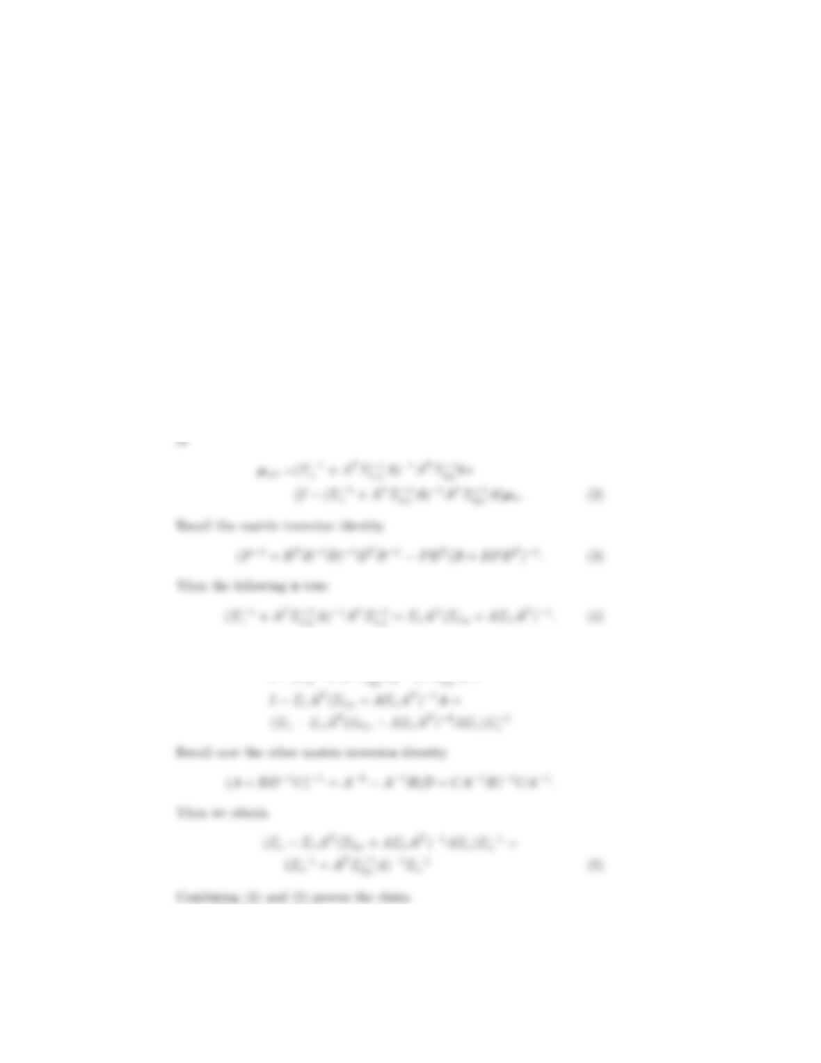
12.1. Show that if
p(z) = N(z|µz, Σz),
and
p(t|z) = N(t|Az, Σt|z),
then
E[z|t] = (Σ−1
z+ATΣ−1
t|zA)−1(ATΣ−1
t|zt+Σ−1
zµz)
Solution: We have shown in the Appendix of the chapter that,
E[z|t] := µz|t=µz+ (Σ−1
z+ATΣ−1
t|zA)−1ATΣ−1
t|z(t−Aµz) (1)
Hence
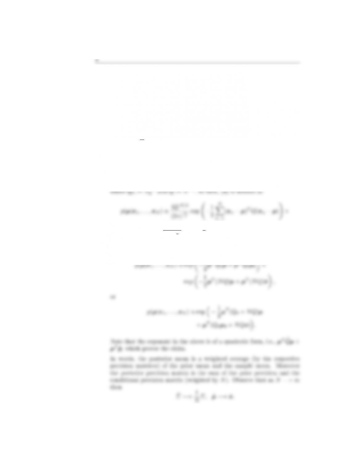
12.2. Let x∈Rlbe a random vector following the normal N(x|µ, Σ). Con-
sider xn, n = 1,2, . . . , N, to be i.i.d. observations. If the prior for µ
follows N(µ|µ0, Σ0), show that the posterior p(µ|x1,...,xN) is normal
N(µ|˜
µ,˜
Σ) with
˜
Σ−1=Σ−1
0+NΣ−1,
and
˜µ=˜
Σ(Σ−1
0µ0+NΣ−1¯
x)
where ¯
x=1
NPN
n=1 xn.
Solution: We have that
p(µ|x1,...,xN)∝p(µ|µ0, Q−1
0)
N
Y
n=1
p(xn|µ;Q−1),(6)
(2π)N l
2
2
n=1
|Q0|1/2
(2π)l
2
exp −1
2(µ−µ0)TQ0(µ−µ0).
Keeping only the terms that depend on µ, we get
NΣ, ˜

12.3. If Xis the set of observed variables and Xlthe set of the corresponding
latent ones, show that
∂ln p(X;ξ)
∂ξ=E∂ln p(X,Xl;ξ)
∂ξ,
where E[·] is with respect to p(Xl|X ;ξ) and ξis an unknown vector pa-
rameter. Note that if one fixes the value of ξin p(Xl|X ;ξ), then one has
obtained the M-step of the EM algorithm.
Solution: we have that
∂ln p(X;ξ)
∂ξ=∂ln R+∞
−∞ p(X,Xl;ξ)dXl
∂ξ
=1
R+∞
−∞ p(X,Xl;ξ)dXl
∂R+∞
−∞ p(X,Xl;ξ)dXl
∂ξ
1
∂p(X,Xl;ξ)
12.4. Show equation (12.42).
Solution: By the definition of Eq. (12.40), in case the hyperparameters
vector is considered to be random, we have,
12.5. Let y∈RN,θ∈Rland Φ a matrix of appropriate dimensions. Derive
the expected value of ky−Φθk2with respect to θ, given E[θ] and the
corresponding covariance matrix Σθ.
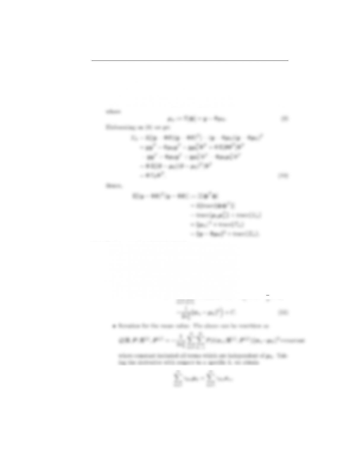
4
Solution: Let φ=y−Φθ. By definition we have
Σφ=E[(φ−E[φ])(φ−E[upφ])T]
=E[φφT]−E[φ]E[φT],(8)
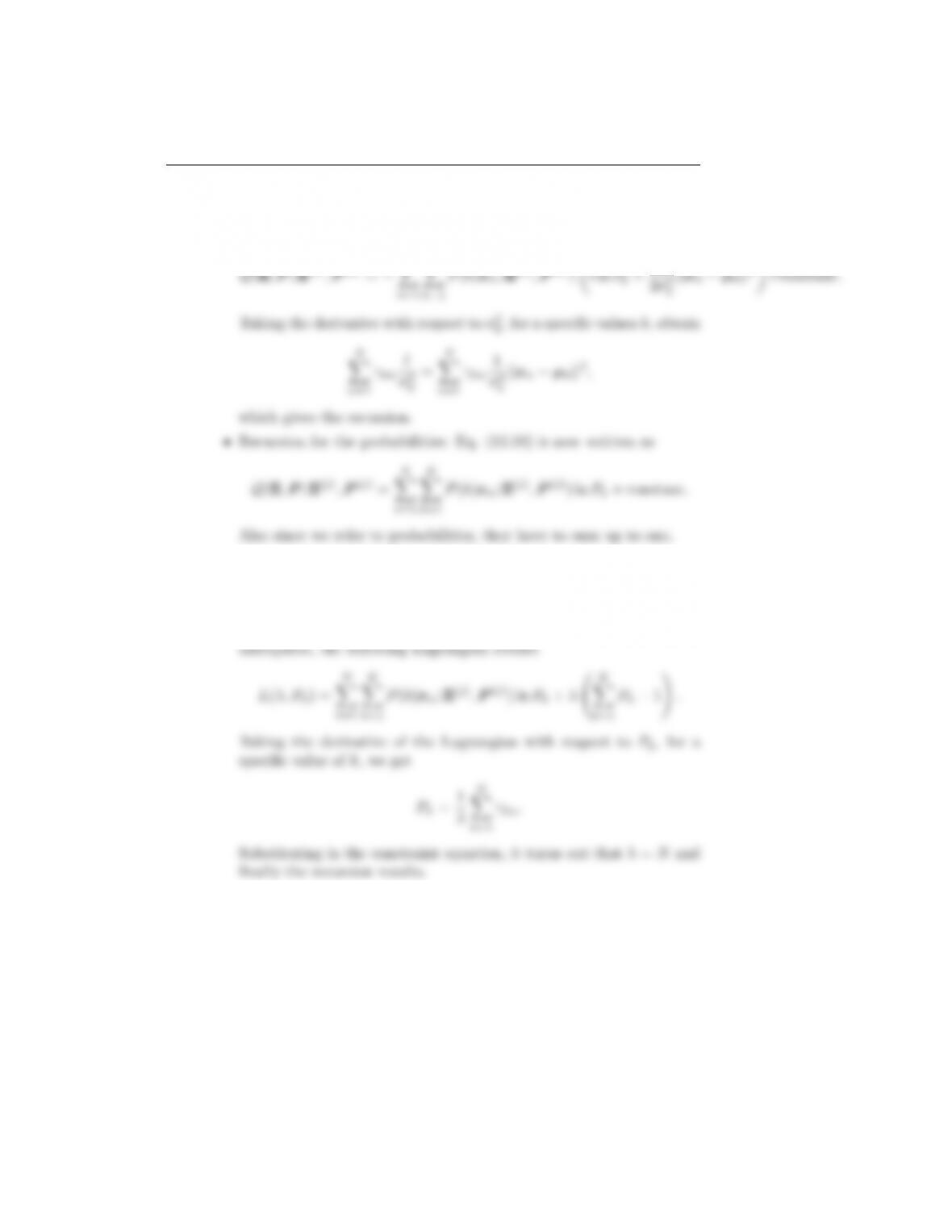
12.6. Derive recursions (12.60)-(12.62).
Solution: Recall from Eq. (12.59) of the text that
Q(Ξ,P;Ξ(j),P(j)) =
N
X
n=1
Ehln p(xn|kn;ξkn)Pkni
:=
N
X
K
X
P(k|xn;Ξ(j),P(j))ln Pk−l
k
n=1
n=1
5
which leads to the recursion.
•Recursion for the variance: Eq. (12.59) is now written as
N
X
K
X
2σ2
K
X
k−1
Pk= 1.
Thus, we have an constrained optimization task. Using Lagrange
12.7. Show that the Kullback-Leibler divergence KL(pkq) is a nonnegative
quantity.
Hint: Recall that ln(·) is a concave function and use Jensen’s inequality,
that is,
fZg(x)p(x)dx≤Zf(g(x))p(x)dx,
where p(x) is a pdf and fis a convex function
6
Solution: By definition of the KL(qkp) divergence and the fact that
−ln(·) is a convex function, we have
KL(qkp) = −Zp(x) ln q(x)
p(x)dx
12.8. Prove that the binomial and beta distributions are conjugate pairs with
respect to the mean value.
Solution: The binomial distribution
12.9. Show that the normalizing constant Cin the Dirichlet pdf
Dir(x|a) = C
K
Y
k=1
xak−1
k,
K
X
k=1
xk= 1,
is given by
C=Γ(a1+a2+. . . +aK)
k=1
k 1−
k=1
7
Solution: We will integrate xK−1out. Then we get
p(x1, x2, . . . , xK−2) =
K−2
Y
k=1 xk
K−1
X
xK−1=t 1−
K−2
X
k=1
xk!.(13)
Hence,
K−2
X
k=1
k 1−
k=1
Z1
0
taK−1−1(1 −t)ak−1dt. (16)
pdf, hence by assumption
CΓ(aK−1)Γ(aK)
Γ(aK−1+aK)=Γ(a1+a2+. . . +aK−2+aK−1+aK)
Γ(α1). . . Γ(αK−2)Γ(aK−1+aK),
or
C=Γ(a1+a2+. . . +aK)
Γ(a1). . . Γ(aK).
12.10. Show that N(x|µ, Σ) for known Σis of an exponential form and that its
conjugate prior is also Gaussian.
Solution:
p(x|µ) = 1
(2π)l/2|Σ|1/2exp −1
2(x−µ)TΣ−1(x−µ)
12.11. Show that the conjugate prior of the multivariate Gaussian with respect
to the precision matrix, Q, is a Wishart distribution.
Solution: We have that,
p(x|Q) = |Q|1/2
(2π)l/2exp −1
2(x−µ)TQ(x−µ)
(2π)l/2exp −1
2[qT
Q:=
qT
1
qT
2
.
.
.
qT
l
and u(x) comprises the columns of (x−µ)(x−µ)T, stacked in sequence
one below the other. Hence p(x|Q) is of an exponential form. Its conjugate
2trace{W−1Q},
which is a Wishart distribution and the normalizing constant then neces-
sarily becomes
l(l−1)
l
Y
j=1
2
−1
12.12. Show that the conjugate prior of the univariate Gaussian N(x|µ, σ2) with
respect to the mean and the precision β=1
σ2, is the Gaussian-gamma
product
p(µ, β;λ, v) = Nµ
v2
λ,(λβ)−1Gamma β
λ+ 1
2,v1
2−v2
2
2λ
where v:= [v1, v2]T.
Solution: We have shown in the respective section in the book that
p(µ, β;λ, v) = h(λ, v)βλ
2exp −λβµ2
2exp [−β
2, βµ]v1
v2,
2β)
2

12.13. Show that the multivariate Gaussian N(x|µ, Q−1) has as a conjugate
prior, with respect to the mean and the precision matrix, Q, the Gaussian-
Wishart product.
Solution: Let
p(x|µ, Q) = |Q|1/2
(2π)l/2exp −1
2µT(λQ)µ−1
2µT
h|Q|ν−λ−1
2exp −1
2trace{W−1Q},
which after some trivial manipulations becomes
2(µ−˜
|Q|˜ν−l−1
2exp −1
2trace{˜
W−1Q},
11
12.14. Show that the distribution
P(x|µ) = µx(1 −µ)1−x, x ∈ {0,1},
is of an exponential form and derive its conjugate prior with respect to µ.
Solution: We have
P(x|µ) = exp ln(µx(1 −µ)1−x)
12.15. Show that estimating an unknown pdf by maximizing the respective en-
tropy, subject to a set of empirical expectations, results in a pdf that
belongs to the exponential family.
Solution: The problem is cast as
maximize w.r.t p(x)ZAx
p(x) ln p(x)dx,
i∈I


