Unlock document.
This document is partially blurred.
Unlock all pages and 1 million more documents.
Get Access
Chapter 18 - Portfolio Performance Evaluation
CHAPTER 18
PORTFOLIO PERFORMANCE EVALUATION
1. a. Possibly. Alpha alone does not determine which portfolio has a larger Sharpe
ratio. Sharpe measure is the primary factor, since it tells us the real return per
unit of risk. We only invest if the Sharpe measure is higher. The standard
b. Yes. It is possible for a positive alpha to exist, but the Sharpe measure declines.
Thus, we would experience inferior performance.
2. Maybe. Provided the addition of funds creates an efficient frontier with the existing
3. No. The M-squared is an equivalent representation of the Sharpe measure, with the
4. Definitely the FF model. Research shows that passive investments (e.g., a market index
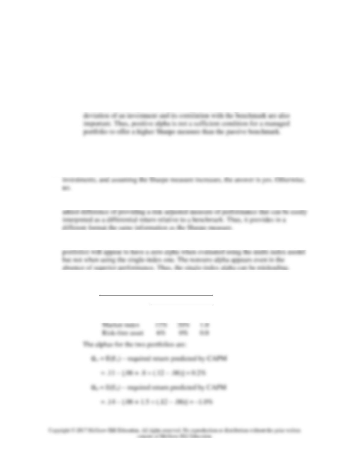
5.
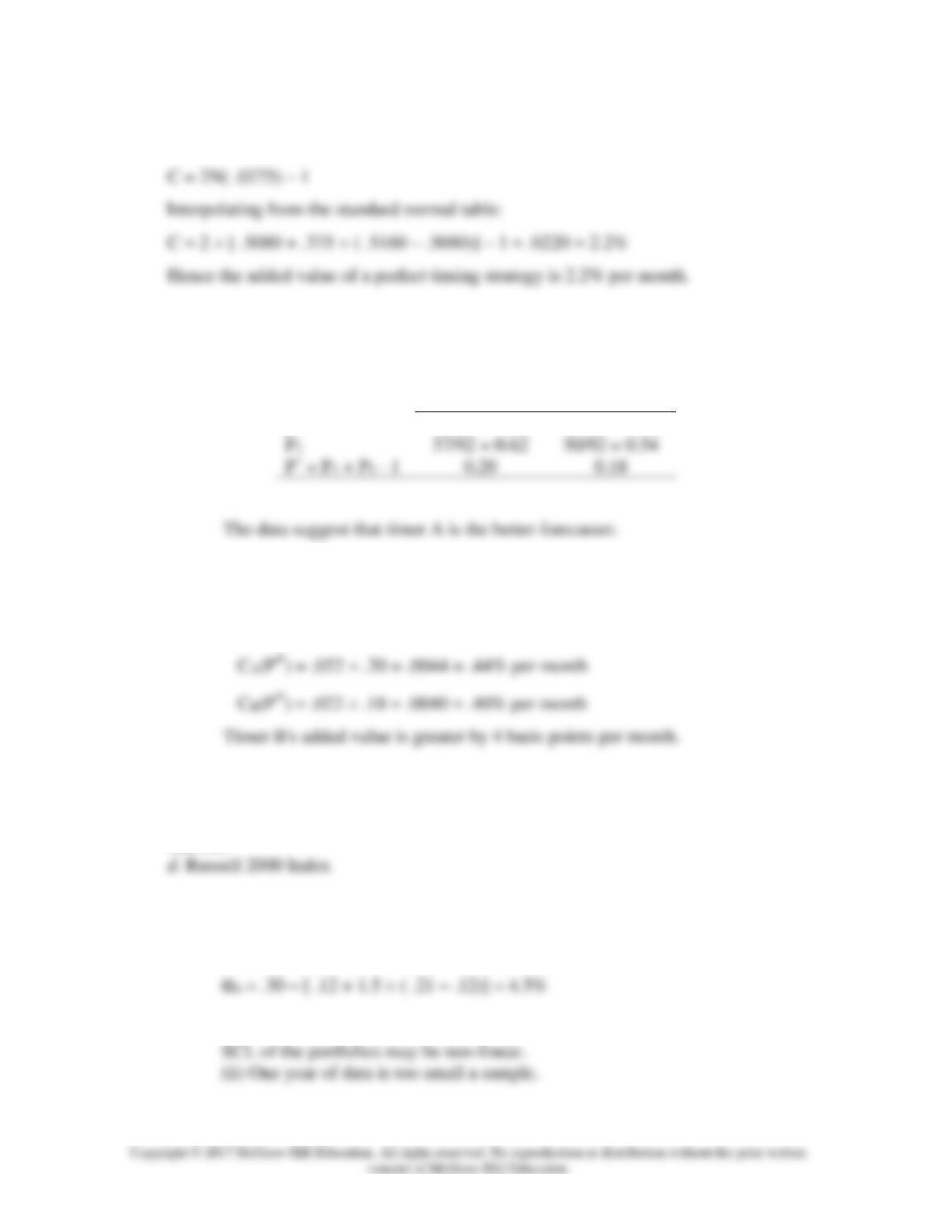
a.
E(r)
Portfolio A
11%
10%
.8
Portfolio B
14%
31%
1.5
Chapter 18 - Portfolio Performance Evaluation
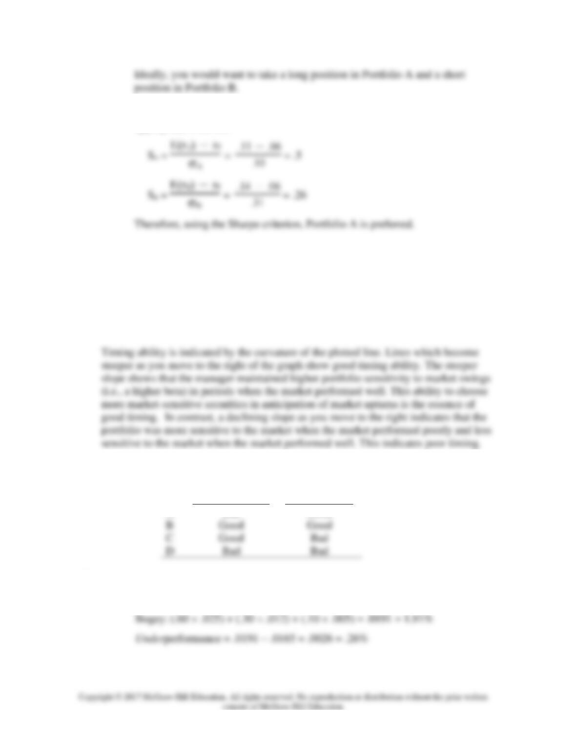
b. If you hold only one of the two portfolios, then the Sharpe measure is the
appropriate criterion:
6. We first distinguish between timing ability and selection ability. The intercept of the
scatter diagram is a measure of stock selection ability. If the manager tends to have a
positive excess return even when the market’s performance is merely “neutral” (i.e., the
market has zero excess return) then we conclude that the manager has, on average,
made good stock picks. In other words, stock selection must be the source of the
positive excess returns.
We can therefore classify performance ability for the four managers as follows:
Selection Ability
Timing Ability
A
Bad
Good
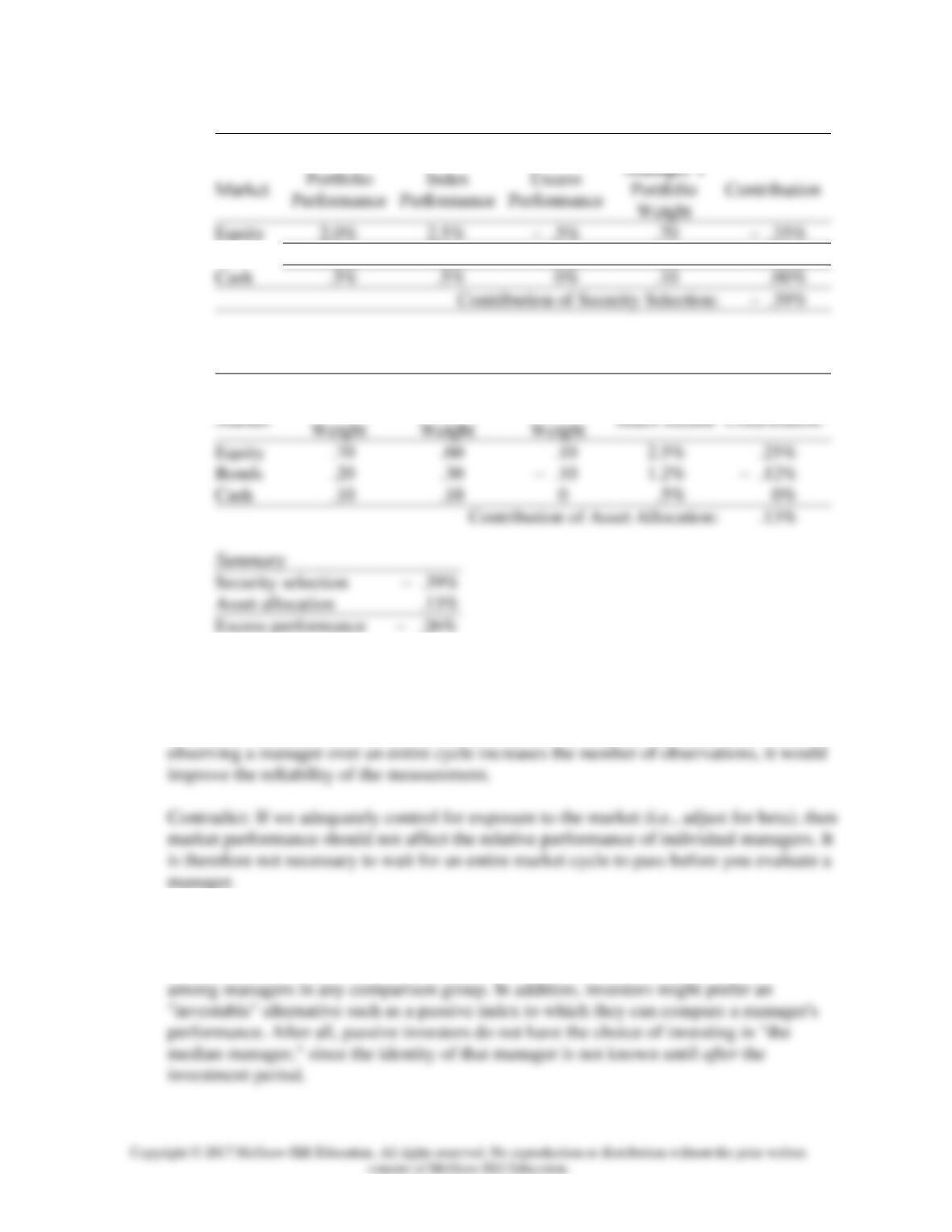
a. Actual: (.70 .02) + (.20 .01) + (.10 .005) = .0165 = 1.65%
Chapter 18 - Portfolio Performance Evaluation
b. Security Selection:
(1)
(2)
(3)
(4)
(5) = (3) (4)
Bonds
1.0%
1.2%
– .2%
.20
– .04%
c. Asset Allocation:
(1)
(2)
(3)
(4)
(5) = (3) (4)
Actual
Benchmark
Excess
8. Support: A manager could be a better forecaster in one scenario than another. For
example, a high-beta manager will do better in up markets and worse in down markets.
Therefore, we should observe performance over an entire cycle. Also, to the extent that
9. It does, to some degree. If those manager groups are sufficiently homogeneous with
respect to style, then relative performance is a decent benchmark. However, one would
like to be able to adjust for the additional variation in style or risk choice that remains
10. The manager’s alpha is: Actual return – Required return predicted by CAPM
11. a. The most likely reason for a difference in ranking is due to the absence of
diversification in Fund A. The Sharpe ratio measures excess return per unit of total
12. The within sector selection calculates the return according to security selection. This is
done by summing the weight of the security in the portfolio multiplied by the return of
the security in the portfolio minus the return of the security in the benchmark:
Selection effect = (Portfolio return – Bogey return) Portfolio weight
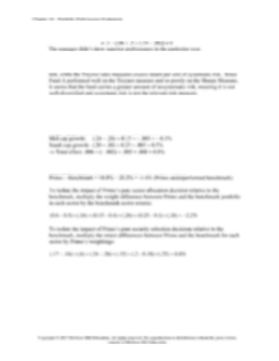
Large-cap growth: (.17 – .16) = =
13. Primo return
0.6 17% 0.15 24% 0.25 20% 18.8%= + + =
Benchmark return
0.5 16% 0.4 26% 0.1 18% 20.2%= + + =
14. Because the passively managed fund is mimicking the benchmark, the
2
R
of the
regression should be very high (and thus probably higher than the actively managed
fund).
15. a. The euro appreciated while the pound depreciated. Primo had a greater stake in the
euro-denominated assets relative to the benchmark, resulting in a positive currency
allocation effect. British stocks outperformed Dutch stocks resulting in a negative
16.
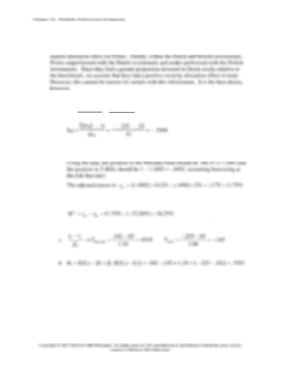
a. SP = E(rP) - rf
P = .102 - .02
.37 = .2216
b. To compute
2
M
measure, blend the Miranda Fund with a position in T-Bills
such that the “adjusted” portfolio has the same volatility as the market index.
Calculate the difference in the adjusted Miranda Fund return and the
benchmark:
[Note: The adjusted Miranda Fund is now 59.46% equity and 40.54% cash.]
17. The spreadsheet below displays the monthly returns and excess returns for the
Vanguard U.S. Growth Fund, the Vanguard U.S. Value Fund and the S&P 500.
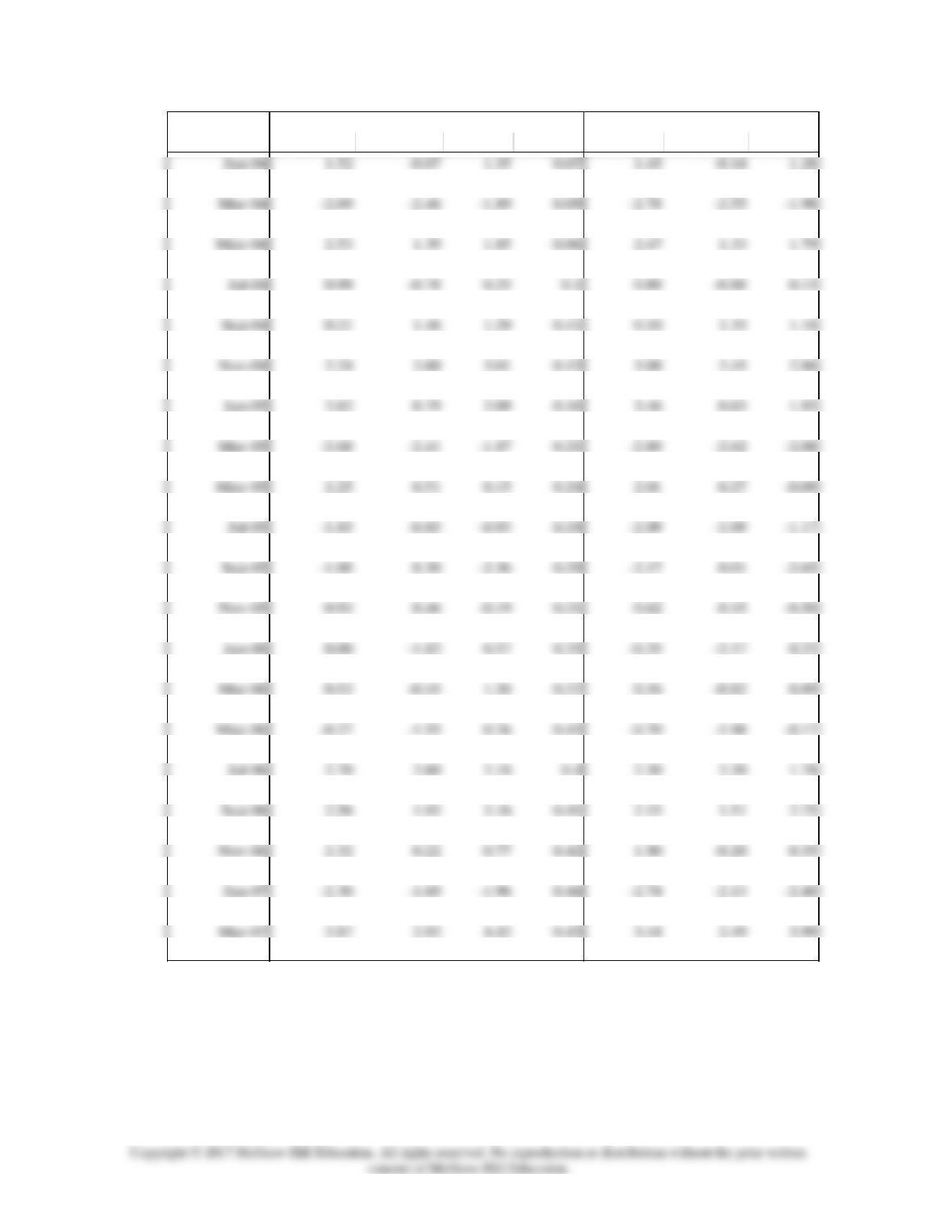
Chapter 18 - Portfolio Performance Evaluation
Total monthly returns Excess Returns
Month Vanguard Value Fund S&P T-bills Vanguard Value Fund S&P
Feb-04 -0.53 -0.99 -1.32 0.06 -0.59 -1.05 -1.38
Apr-04 0.22 2.52 1.70 0.08 0.14 2.44 1.62
Jun-04 -1.93 -7.46 -3.22 0.08 -2.01 -7.54 -3.30
Aug-04 1.52 2.49 1.00 0.11 1.41 2.38 0.89
Oct-04 5.22 4.66 4.46 0.11 5.11 4.55 4.35
Dec-04 -2.36 -3.48 -2.24 0.16 -2.52 -3.64 -2.40
Feb-05 -2.33 -2.86 -1.83 0.16 -2.49 -3.02 -1.99
Apr-05 4.08 7.13 3.22 0.21 3.87 6.92 3.01
Jun-05 3.55 5.28 3.82 0.23 3.32 5.05 3.59
Aug-05 0.38 1.34 0.80 0.3 0.08 1.04 0.50
Oct-05 2.87 5.04 4.39 0.27 2.60 4.77 4.12
Dec-05 3.41 3.30 2.41 0.32 3.09 2.98 2.09
Feb-06 0.71 0.34 1.65 0.34 0.37 0.00 1.31
Apr-06 -3.00 -5.84 -3.01 0.36 -3.36 -6.20 -3.37
Jun-06 1.09 -2.36 0.45 0.4 0.69 -2.76 0.05
Aug-06 2.63 2.87 2.70 0.42 2.21 2.45 2.28
Oct-06 0.75 1.94 1.99 0.41 0.34 1.53 1.58
Dec-06 1.86 2.18 1.51 0.4 1.46 1.78 1.11
Feb-07 0.81 0.89 1.16 0.38 0.43 0.51 0.78
Apr-07 3.65 3.37 3.39 0.44 3.21 2.93 2.95
Chapter 18 - Portfolio Performance Evaluation
Jun-07 -4.74 -0.79 -3.13 0.4 -5.14 -1.19 -3.53
Aug-07 2.54 4.91 3.88 0.42 2.12 4.49 3.46
Oct-07 -5.86 -3.90 -3.87 0.32 -6.18 -4.22 -4.19
Dec-07 -5.39 -10.34 -6.04 0.27 -5.66 -10.61 -6.31
Feb-08 -0.89 -0.06 -0.90 0.13 -1.02 -0.19 -1.03
Apr-08 1.44 3.00 1.51 0.17 1.27 2.83 1.34
Jun-08 -1.80 -0.40 -0.90 0.17 -1.97 -0.57 -1.07
Aug-08 -7.50 -11.63 -9.42 0.12 -7.62 -11.75 -9.54
Oct-08 -7.16 -7.93 -6.96 0.08 -7.24 -8.01 -7.04
Dec-08 -10.76 -4.49 -8.22 0.09 -10.85 -4.58 -8.31
Average -0.59 -0.60 -0.55
bSD 4.05 4.21 3.81
c Beta 1.03 1.02 1.00
a. The excess returns are noted in the spreadsheet.
d. The formulas for the three measures are below and results listed above.
Sharpe: E(rP) - rf
P
Chapter 18 - Portfolio Performance Evaluation
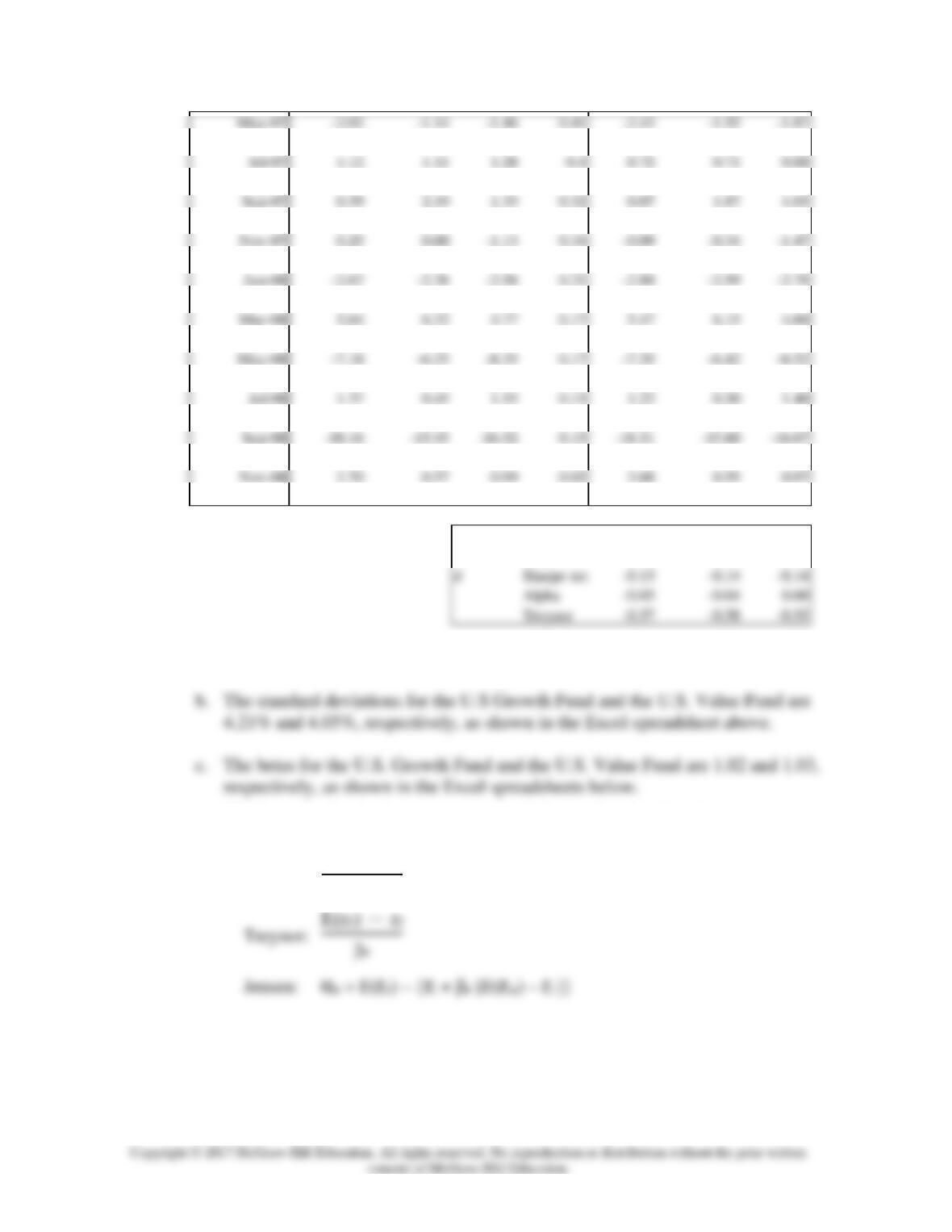
SUMMARY OUTPUT Vanguard
Regression Statistics
Multiple R 0.97
ANOVA
df SS MS F
Regression 1.00 907.97 907.97 876.67
Coefficients Standard Error t Stat P-value
SUMMARY OUTPUT Value Fund
Regression Statistics
Multiple R 0.93
R Square 0.86
ANOVA
df SS MS F
Regression 1.00 896.12 896.12 343.89
Coefficients Standard Error t Stat P-value
Intercept (0.04) 0.21 (0.17) 0.86
18. See the Black-Scholes formula. Substitute:
Current stock price = S0 = $1.0
Exercise price = X = (1 + rf) = 1.01
Standard deviation = = .055
Chapter 18 - Portfolio Performance Evaluation
N(/2) is the cumulative standard normal density for the value of half the standard
deviation of the equity portfolio.
19.
a. Using the relative frequencies to estimate the conditional probabilities P1 and P2
for timers A and B, we find:
Timer A
Timer B
P1
78/135 = 0.58
86/135 = 0.64
b. Use the following equation and the previous answer to value the imperfect timing
services of Timer A and Timer B:
C(P*) = C(P1 + P2 – 1)
CFA 1
Answer:
CFA 2
Answer:
a. αA = .24 – [ .12 + 1.0 ( .21 – .12)] = 3.0%
b. (i) The managers may have been trying to time the market. In that case, the
Chapter 18 - Portfolio Performance Evaluation
CFA 3
Answer:
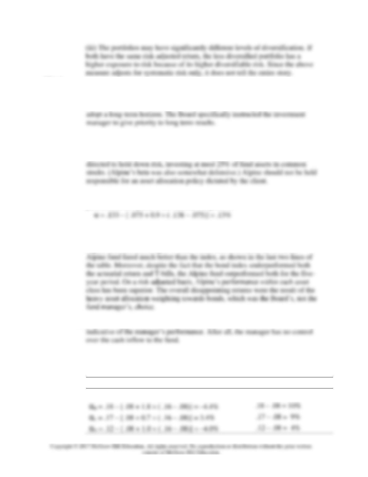
a. Indeed, the one year results were terrible, but one year is a poor statistical base
from which to draw inferences. Moreover, the fund manager was directed to
b. The sample of pension funds held a much larger share in equities compared to
the Alpine pension fund. The stock and bond indexes indicate that equity returns
significantly exceeded bond returns. The Alpine fund manager was explicitly
c. Over the five-year period, Alpine’s alpha, which measures risk-adjusted
performance compared to the market, was positive:
d. Note that, over the last five years, and particularly the last one year, bond
performance has been poor; this is significant because this is the asset class that
Alpine had been encouraged to hold. Within this asset class, however, the
e. A trustee may not care about the time-weighted return, but that return is more
CFA 4
Answer:
a.
Alpha (): αi = E(ri) – {rf + βi [E(rM) – rf ]}
Expected excess return: E(ri) – rf
αA = .20 – [ .08 + 1.3 ( .16 – .08)] = 1.6%
.20 – .08 = 12%
Chapter 18 - Portfolio Performance Evaluation
Stocks A and C have positive alphas, whereas stocks B and D have negative
alphas.
The residual variances are:
2(eA) = .582 = .3364
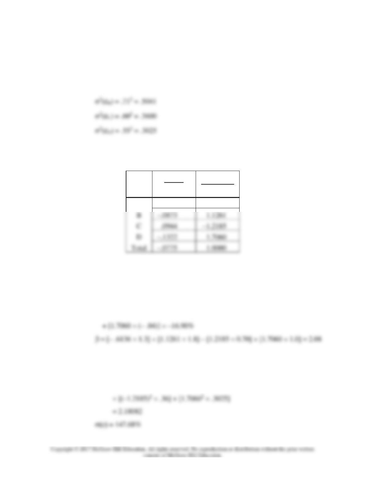
b. To construct the optimal risky portfolio, we first determine the optimal active
portfolio. Using the Treynor-Black technique, we construct the active
portfolio:
2(e)
2(e)
αi2(ei)
A
.0476
–0.6136
Do not be disturbed by the fact that the positive alpha stocks get negative
weights and vice versa. The entire position in the active portfolio will turn out
to be negative, returning everything to good order.
With these weights, the forecast for the active portfolio is:
α = [– .6136 .016] + [1.1261 (– .044)] – [1.2185 .034]
The high beta (higher than any individual beta) results from the short positions
in the relatively low beta stocks and the long positions in the relatively high
beta stocks.
2(e) = [(– .6136)2 .3364] + [1.12612 .5041]
Chapter 18 - Portfolio Performance Evaluation
Here, again, the levered position in stock B [with the high 2(e)] overcomes the
diversification effect, and results in a high residual standard deviation. The
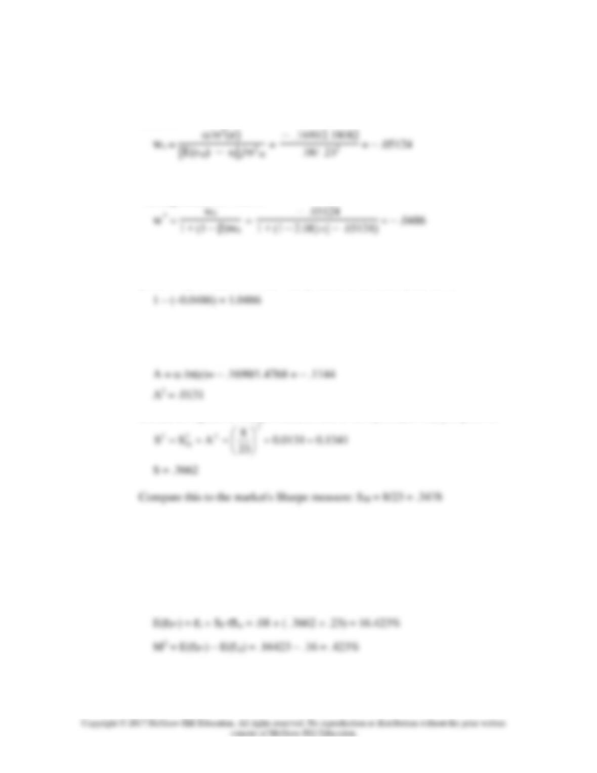
optimal risky portfolio has a proportion w* in the active portfolio, computed as
follows:
The negative position is justified for the reason given earlier.
The adjustment for beta is:
Because w* is negative, we end up with a positive position in stocks with
positive alphas and vice versa. The position in the index portfolio is:
c. To calculate Sharpe's measure for the optimal risky portfolio we compute the
appraisal ratio for the active portfolio and Sharpe's measure for the market
portfolio. The appraisal ratio of the active portfolio is:
Hence, the square of Sharpe's measure (S) of the optimized risky portfolio is:
The difference is: .0184
Note that the only-moderate improvement in performance results from the fact
that only a small position is taken in the active portfolio A because of its large
residual variance.
We calculate the "Modigliani-squared" (M2) measure, as follows:


